Ngô Quốc Anh

August 16, 2009

On the stability of the Runge-Kutta 4 (RK4)


In the literature, the so-called RK4 is given as following: we first define the following coefficients
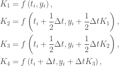
\displaystyle \begin{gathered}{K_{1}}= f\left({{t_{i}},{y_{i}}}\right),\hfill\\ {K_{2}}= f\left({{t_{i}}+\frac{1}{2}\Delta t,{y_{i}}+\frac{1}{2}\Delta t{K_{1}}}\right),\hfill\\ {K_{3}}= f\left({{t_{i}}+\frac{1}{2}\Delta t,{y_{i}}+\frac{1}{2}\Delta t{K_{2}}}\right),\hfill\\ {K_{4}}= f\left({{t_{i}}+\Delta t,{y_{i}}+\Delta t{K_{3}}}\right),\hfill\\ \end{gathered}

then

\displaystyle {y_{i + 1}} = {y_i} + \frac{{\Delta t}} {6}\left( {{K_1} + 2{K_2} + 2{K_3} + {K_4}} \right).

This is the most important iterative method for the approximation of solutions of ordinary differential equations

\displaystyle y' = f(t, y), \quad y(t_0) = y_0.

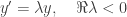
This technique was developed around 1900 by the German mathematicians C. Runge and M.W. Kutta. In order to study its stability, we use the model problem

\displaystyle y' = \lambda y, \quad \Re \lambda < 0.

In other words, we replace f(t,y) by \lambda y. Then the stability condition for time step \Delta comes from the following condition

\displaystyle \left| \frac{y_{i+1}}{y_i} \right| \leq 1.

Applying the above discussion to RK4 method, we see that

\displaystyle\begin{gathered}{K_{4}}=\lambda\left({{y_{i}}+\Delta t{K_{3}}}\right),\hfill\\ {K_{3}}=\lambda\left({{y_{i}}+\frac{1}{2}\Delta t{K_{2}}}\right),\hfill\\ {K_{2}}=\lambda\left({{y_{i}}+\frac{1}{2}\Delta t{K_{1}}}\right),\hfill\\ {K_{1}}=\lambda{y_{i}},\hfill\\ \end{gathered}

which implies

\displaystyle\begin{gathered}{K_{4}}=\lambda\left({{y_{i}}+\Delta t\lambda\left({{y_{i}}+\frac{1}{2}\Delta t\lambda\left({{y_{i}}+\frac{1}{2}\Delta t{y_{i}}}\right)}\right)}\right) =\lambda{y_{i}}\left({1+\Delta t\lambda\left({1+\frac{1}{2}\Delta t\lambda\left({1+\frac{1}{2}\Delta t}\right)}\right)}\right),\hfill\\ {K_{3}}=\lambda\left({{y_{i}}+\frac{1}{2}\Delta t\lambda\left({{y_{i}}+\frac{1}{2}\Delta t{y_{i}}}\right)}\right) =\lambda{y_{i}}\left({1+\frac{1}{2}\Delta t\lambda\left({1+\frac{1}{2}\Delta t}\right)}\right),\hfill\\ {K_{2}}=\lambda\left({{y_{i}}+\frac{1}{2}\Delta t\lambda{y_{i}}}\right) =\lambda{y_{i}}\left({1+\frac{1}{2}\Delta t\lambda }\right),\hfill\\ {K_{1}}=\lambda{y_{i}},\hfill\\ \end{gathered}

which yields

\displaystyle\begin{gathered}{K_{4}}=\lambda\left({{y_{i}}+\Delta t\lambda\left({{y_{i}}+\frac{1}{2}\Delta t\lambda\left({{y_{i}}+\frac{1}{2}\Delta t{y_{i}}}\right)}\right)}\right) =\lambda{y_{i}}\left({1+\Delta t\lambda\left({1+\frac{1}{2}\Delta t\lambda\left({1+\frac{1}{2}\Delta t}\right)}\right)}\right),\hfill\\ {K_{3}}=\lambda\left({{y_{i}}+\frac{1}{2}\Delta t\lambda\left({{y_{i}}+\frac{1}{2}\Delta t{y_{i}}}\right)}\right) =\lambda{y_{i}}\left({1+\frac{1}{2}\Delta t\lambda\left({1+\frac{1}{2}\Delta t}\right)}\right),\hfill\\ {K_{2}}=\lambda\left({{y_{i}}+\frac{1}{2}\Delta t\lambda{y_{i}}}\right) =\lambda{y_{i}}\left({1+\frac{1}{2}\Delta t\lambda }\right),\hfill\\ {K_{1}}=\lambda{y_{i}},\hfill\\ \end{gathered}

Thus

\displaystyle\frac{{{y_{i+1}}}}{{{y_{i}}}}= 1+\frac{{\Delta t}}{6}\left[{\lambda+2\lambda\left({1+\frac{1}{2}\Delta t\lambda }\right)+2\lambda\left({1+\frac{1}{2}\Delta t\lambda\left({1+\frac{1}{2}\Delta t}\right)}\right)+\lambda\left[{1+\Delta t\lambda\left({1+\frac{1}{2}\Delta t\lambda\left({1+\frac{1}{2}\Delta t}\right)}\right)}\right]}\right]

which is nothing but

\displaystyle\frac{{{y_{i+1}}}}{{{y_{i}}}}= 1+\Delta t\lambda+\frac{{{{\left({\Delta t\lambda }\right)}^{2}}}}{2}+\frac{{{{\left({\Delta t\lambda }\right)}^{3}}}}{6}+\frac{{{{\left({\Delta t\lambda }\right)}^{4}}}}{{24}}.

Therefore, the stability condition is given as follows

\displaystyle \left| {1 + z + \frac{{{z^2}}} {2} + \frac{{{z^3}}} {6} + \frac{{{z^4}}} {{24}}} \right| \leq 1, \quad \Re z < 0.

The eigenvalues of a common tridiagonal matrix

Filed under: Các Bài Tập Nhỏ, Linh Tinh, Nghiên Cứu Khoa Học — Ngô Quốc Anh @ 3:36

The eigenvalues of then N \times N tridiagonal matrix

\left( {\begin{array}{*{20}{c}}    a & b & {} & {} & {} & {} & {}  \\    c & a & b & {} &...

are

{\lambda _s} = a + 2\sqrt {bc} \cos \frac{{s\pi }} {{N + 1}}

and its conresponding eigenvector is

{v_s}^T = \left( {{{\left( {\frac{c} {b}} \right)}^{\frac{1} {2}}}\sin \frac{{s\pi }} {{N + 1}},{{\left( {\frac{c} {b}} \righ...

Proof. Let \lambda present an eigenvalue of the given matrix (denoted by A) and v the corresponding eigenvector with components v_1,...,v_N. Then

\left( {\begin{array}{*{20}{c}}    a & b & {} & {} & {} & {} & {}  \\    c & a & b & {} &...

If we defined v_0 = v_{N+1}=0, then we have

c{v_{i - 1}} + \left( {a - \lambda } \right){v_i} + b{v_{i + 1}} = 0,i = \overline {1,N} .

The solution of the above equation is of the form

{v_i} = Bm_1^i + Cm_2^i

where B, C are constants and m_1, m_2 are the roots of the equation

c+(a-\lambda)m + bm^2=0.

Since v_0 = v_{N+1}=0, then 0=B+C and 0 = Bm_1^{N + 1} + Cm_2^{N + 1}. Hence,

{\left( {\frac{{{m_1}}} {{{m_2}}}} \right)^{N + 1}} = 1 = {e^{\sqrt { - 1} i2\pi }}

or

\frac{{{m_1}}} {{{m_2}}} = {e^{\frac{{\sqrt { - 1} i2\pi }} {{N + 1}}}}.

We also have

{m_1}{m_2} = \frac{c} {b}, \quad {m_1} + {m_2} = \frac{{\lambda  - a}} {b}.

Finally,

\lambda  = a + b\sqrt {\frac{c} {b}} \left( {{e^{\frac{{\sqrt { - 1} i2\pi }} {{N + 1}}}} + {e^{ - \frac{{\sqrt { - 1} i2\pi ...

The j-component of the eigenvector is

{v_j} = Bm_1^j + Cm_2^j = B\sqrt {{{\left( {\frac{c} {b}} \right)}^j}} \left( {{e^{\frac{{\sqrt { - 1} i2\pi }} {{N + 1}}}} -...

Blog at WordPress.com.