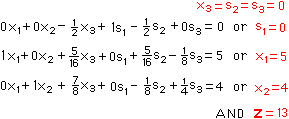
Linear Least Square Problem (linear least squares), or ordinary least squares (OLS), is an important computational problem, that arises primarily in applications when it is desired to fit a linear mathematical model to measurements obtained from experiments. The goals of linear least squares are to extract predictions from the measurements and to reduce the effect of measurement errors. Mathematically, it can be stated as the problem of finding an approximate solution to an overdetermined system of linear equations. In statistics, it corresponds to the maximum likelihood estimate for a linear regression with normally distributed error.
Linear least square problems admit a closed-form solution, in contrast to non-linear least squares problems, which often have to be solved by an iterative procedure.
Motivational example
As a result of an experiment, four  data points were obtained,
  ,
,  ,
,  , and
, and  (shown in red in the picture on the right). It is desired to find a line
  that fits “best” these four points. In other words, we would like to find the numbers
  and
and  that approximately solve the overdetermined linear system
 .
.
of four equations in two unknowns in some “best” sense.

The least squares approach to solving this problem is to try to make as small as possible the sum of squares of “errors” between the right- and left-hand sides of these equations, that is, to find the minimum of the function
![\displaystyle S(\beta_1, \beta_2)= \left[6-(\beta_1+1\beta_2)\right]^2 +\left[5-(\beta_1+2\beta_2) \right]^2 +\left[7-(\beta_1 + 3\beta_2)\right]^2 +\left[10-(\beta_1 + 4\beta_2)\right]^2](https://s0.wp.com/latex.php?latex=%5Cdisplaystyle+S%28%5Cbeta_1%2C+%5Cbeta_2%29%3D+%5Cleft%5B6-%28%5Cbeta_1%2B1%5Cbeta_2%29%5Cright%5D%5E2+%2B%5Cleft%5B5-%28%5Cbeta_1%2B2%5Cbeta_2%29+%5Cright%5D%5E2+%2B%5Cleft%5B7-%28%5Cbeta_1+%2B+3%5Cbeta_2%29%5Cright%5D%5E2+%2B%5Cleft%5B10-%28%5Cbeta_1+%2B+4%5Cbeta_2%29%5Cright%5D%5E2&bg=ffffff&fg=333333&s=0&c=20201002) .
.
The minimum is determined by calculating the partial derivatives of  in respect to and and setting them to zero. This results in a system of two equations in two unknowns, called the normal equations, which, when solved, gives the solution

and the equation  of the line of best fit. The residuals, that is, the discrepancies between the
  values from the experiment and the values calculated using the line of best fit are then found to be
  ,
,  ,
,  , and
, and  (see the picture on the right). The minimum value of the sum of squares is
 .
.
The general problem
Consider an overdetermined system (there are more equations than unknowns)
 ,
,
of  linear equations in n unknown coefficients, ,,…,
 , with
  , written in matrix form as
  ,where
 .
.
Such a system usually has no solution, and the goal is then to find the coefficients  which fit the equations “best”, in the sense of solving the quadratic minimization problem.
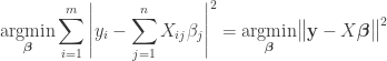 .
.
A justification for choosing this criterion is given in properties below. This minimization problem has a unique solution, provided that the  columns of the matrix
  are linearly independent, given by solving the normal equations
 .
.
Singular value decomposition
In linear algebra, the singular value decomposition (SVD) is an important factorization of a rectangular real or complex matrix, with many applications in signal processing and statistics. Applications which employ the SVD include computing the pseudo-inverse, least squares fitting of data, matrix approximation, and determining the rank, range and null space of a matrix.
Suppose  is an -by- matrix whose entries come from the field
  , which is either the field of real numbers or the field of complex numbers. Then there exists a factorization of the form
 ,
,
where  is an -by- unitary matrix over , the matrix
  is -by- diagonal matrix with nonnegative real numbers on the diagonal, and
  denotes the conjugate transpose of
  , an -by- unitary matrix over . Such a factorization is called a singular-value decomposition of . A common convention is to order the diagonal entries
  in non-increasing fashion. In this case, the diagonal matrix is uniquely determined by (though the matrices and are not). The diagonal entries of are known as the singular values of .
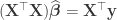
In practice, matrix consists of eigenvectors of matrix  while matrix consists of eigenvectors of matrix
  . Finally, matrix is the square root of a diagonal matrix forming by eigenvalues of either matrix or matrix .
Example
Let us consider the case when
 .
.
Having  yields

and
 .
.
By simple calculation, one has

being eigenvalues of matrix  (in the descending form), which helps us to write down

To construct matrix  , one has to find eigenvectors corresponding to eigenvalues
  and
and  . For the first one, that is, , one has the following linear system

which implies, for example,
 .
.
Similar to , one has its corresponding eigenvector as follows
 .
.
Thus
 .
.
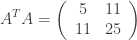
The numerical solution of is

which gives us
 .
.
Having we can compute by the following formula  or you can perform the same routine as above. That is
 .
.
It is easy to see that
 .
.
Having a SVD result, that is
one can see that the solution of  can be computed by
 .
.
Note that matrices and are not unique. Using Maple software, you can compute SVD as shown below.

Useful links


 (
( ) are the inequality constraints and
  (
( ) are the equality constraints, and
  are the number of inequality and equality constraints, respectively.
 and the constraint functions are
  and
and  . Further, suppose they are continuously differentiable at a point
  . If
. If  and
and  such that
 ,
,
 .
. .
. .
. ) is positive-linear dependent if there exists
  ,…,
,…, not all zero such that
  ).
). for equalities and
  for inequalities than it doesn’t exist a sequence
  such that
  therefore
  and
and  thus
thus  .
. such that
  and
and  for all
  active in
  and
and  are affine functions, then no other condition is needed to assure that the minimum point is KKT.
 are continuously differentiable convex functions and the equality constraints hi are affine functions. It was shown by Martin in 1985 that the broader class of functions in which KKT conditions guarantees global optimality are the so called invex functions. So if equality constraints are affine functions, inequality constraints and the objective function are continuously differentiable invex functions then KKT conditions are sufficient for global optimality.

 .
. .)
.) increases. Thus if each
  ,
,  with
with  .
.![[a,b]](https://i0.wp.com/alt1.mathlinks.ro/latexrender/pictures/1/4/7/1475c39442659c6febe03b2e1809dbde6ec5fb5a.gif) into
into  subintervals by the following interior points
  .
.  . T
. T , which will be denoted by
  , is called the step size. The value of
  at step
  is usually denoted by
  , that is,
  .
.  . T
. T , we can compute the value of
  by using the following scheme
 ,
,  , constants.
 th-order system of 1st initial value problems has the form
 ,
,  ,…,
,…, .
.  . We denote by
  the following number
 , having all
  for all
  . To do this, for each
  ,
,  . More precisely, we need to compute
 and for each
 , with
  .
.
 and
and  by using the following scheme
 decomposition (also called a
  is a decomposition of
  where
where  is an orthogonal matrix (meaning that
  ) and
) and  is an upper triangular matrix (also called right triangular matrix). This generalizes to a complex square matrix
  matrix
  , as the product of an
  unitary matrix
  rows of an
 is an
is an  upper triangular matrix,
  is
is  is
is  , and
, and  the thin
  and we require that the diagonal elements of
  (
( if
if  ,
,  and
and  decompositions
  being a lower triangular matrix.
 , one can solve the Least Square Problem
  where
where  and
and  with
with  . To be precise, by mean of
 ![Q = \left( {\begin{array}{*{20}{c}} {{{\left[ {{Q_1}} \right]}_{m \times n}}} & {{{\left[ {{Q_2}} \right]}_{m \times \...](https://i0.wp.com/alt2.mathlinks.ro/latexrender/pictures/d/1/7/d177fe503a9df3ceca3374824c92382e0a3a61d6.gif)
 . Thus
  .
.  . Assume that after finishing the Gram–Schmidt process, we obtain
  . Therefore, we put
 .
.

 , we obtain
  from
from  , that is,
 , we firstly project
  onto
onto 


![\{|z|^2<1,I[z]>0\}](https://s0.wp.com/latex.php?latex=%5C%7B%7Cz%7C%5E2%3C1%2CI%5Bz%5D%3E0%5C%7D&bg=ffffff&fg=333333&s=0&c=20201002) . Further suppose that
. Further suppose that 
 reflected across the real axis are the reflections of
  across the real axis. It is easy to check that the above function is complex differentiable in the interior of the lower half-disk. What is remarkable is that the resulting function must be analytic along the real axis as well, despite no assumptions of differentiability.
 .
.
 to a harmonic function on the reflected domain. Again note that it is necessary for
  . This result provides a way of extending a harmonic function from a given open set to a larger open set (Krantz 1999, p. 95).
 is a small perturbation on
  is a small perturbation on
  holds true. This together with the fact that
  gives
gives  . By some simple calculation, one has
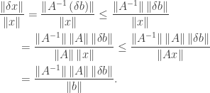

 is a small perturbation on
  holds true. This together with the fact that
  . By some simple calculation, one has


 holds true. This together with the fact that
  . By some simple calculation, one has

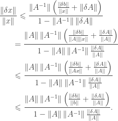
 is called the condition number of the matrix
  . It is easy to see that
  . If
. If  , the system
  represent the difference equation approximating the PDE at the
  -th mesh point, with exact solution
  . For example,

 -th mesh point. If
  , where
  is called the local truncation error
  at the
  .
. .
. and
and  and partial derivatives of
  represent the PDE in the independent variables
  , with exact solution
  represent the approximating finite-difference equation with exact solution
  to be evaluated at the point
  .
. at the point
  .
. as
as  and
and  , the difference equation is said to be consistent or compatible with the PDE. Most authors put
  because

 ,
, and
and  .
. into
into  parts and the domain
  into
into  .
.
 . At
. At  , that is
  , one has
 , that is
  , one obtains
 .
.
 with the following boundary conditions


 .
.