Ngô Quốc Anh

January 14, 2013

Hyperbolicity of the 3+1 system of the Einstein equations under the harmonic slicing

Filed under: Uncategorized — Tags: — Ngô Quốc Anh @ 2:20

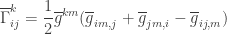
Let us first recall the evolution equation of K in this note

\displaystyle \frac{\partial }{{\partial t}}{K_{\alpha \beta }} = - {\nabla _\alpha }{\nabla _\beta }N + N({\text{Ric}_{\alpha \beta }}-\gamma _\alpha ^\mu \gamma _\beta ^\nu {\overline {\text{Ric}} _{\mu \nu }} + K{K_{\alpha \beta }} - 2{K_{\alpha \mu }}K_\beta ^\mu ) + {\mathcal L_{\vec \beta}}{K_{\alpha \beta }},

which can be rewritten as the following

\displaystyle {\overline {{\text{Ric}}} _{\alpha \beta }} = - \frac{1}{N}{\nabla _\alpha }{\nabla _\beta }N + {\text{Ri}}{{\text{c}}_{\alpha \beta }} + K{K_{\alpha \beta }} - 2{K_{\alpha \mu }}K_\beta ^\mu - \frac{1}{N}(\frac{\partial }{{\partial t}} - {\mathcal{L}_{\vec \beta }}){K_{\alpha \beta }}

for all \alpha ,\beta > 0 since in our setting \gamma_i^j=\delta_i^j for all i,j>0. The quantities \text{Ric}_{0\beta} and \text{Ric}_{00} come from the Codazzi and Ricci equations. To be precise, we have, by the Codazzi equation,

\displaystyle {\overline {{\text{Ric}}} _{0\beta }} = {\nabla _h}K_\beta ^h - {\partial _\beta }K

and, by the Ricci equation,

\displaystyle {\overline {{\text{Ric}}} _{00}} = \frac{1}{N}(\frac{\partial }{{\partial t}} - {\mathcal{L}_{\vec \beta }})K + \frac{1}{N}{\nabla ^i}{\nabla _i}N + {K_{ij}}{K^{ij}}.

It is clear that the infinitesimal variation of the Ricci curvature \delta R_{mu\nu} corresponding to an infinitesimal \delta g variation of the space metric is

\displaystyle\delta {R_{\mu \nu }} = \frac{1}{2}({\nabla ^h}{\nabla _{(i}}\delta {g_{j)h}} - {\nabla _h}{\nabla ^h}\delta {g_{ij}} - {\nabla _j}{\partial _i}({g^{hk}}\delta {g_{hk}})),

where the notation (i j) is nothing but ij+ji. This formula can be applied to \frac{\partial}{\partial t} and \mathcal L_{\vec \beta} to get

\displaystyle (\frac{\partial }{{\partial t}} - {\mathcal{L}_{\vec \beta }}){R_{\mu \nu }} = \frac{1}{2} \Big({\nabla ^h}{\nabla _{(i}}(\frac{\partial }{{\partial t}} - {\mathcal{L}_{\vec \beta }}){g_{j)h}} - {\nabla _h}{\nabla ^h}(\frac{\partial }{{\partial t}} - {\mathcal{L}_{\vec \beta }}){g_{ij}} - {\nabla _j}{\partial _i}({g^{hk}}(\frac{\partial }{{\partial t}} - {\mathcal{L}_{\vec \beta }}){g_{hk}}) \Big).

(more…)

January 11, 2013

The stress-energy tensor and Einstein constraint equations in the presence of scalar fields

Filed under: Uncategorized — Tags: — Ngô Quốc Anh @ 6:26

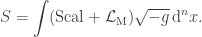
In this notes, we are particularly interested in some special model of general relativity. More precisely, here we consider the scalar fields since, for example, a real scalar field more or less provides one of the simplest sources of stress-energy in GR.

1. Derivation of stress-energy tensor.

To derive the stress-energy tensor associated to a real scalar field, we make use of the Einstein-Hilbert action. Suppose that the full action of the theory is given by the Einstein–Hilbert term plus a term \mathcal{L}_\mathrm{M} describing any matter fields appearing in the theory, then we have

\displaystyle S = \int ( \text{Scal} + \mathcal{L}_\mathrm{M} ) \sqrt{-g}\, \mathrm{d}^n x .

The action principle then tells us that the variation of this action with respect to the inverse metric is zero, yielding \delta S=0. Calculating this equation gives

\displaystyle \frac{\delta R}{\delta g^{\mu\nu}} + \frac{R}{\sqrt{-g}} \frac{\delta \sqrt{-g}}{\delta g^{\mu\nu}} =-2 \frac{\delta \mathcal{L}_\mathrm{M}}{\delta g^{\mu\nu}} + g_{\mu\nu} \mathcal{L}_\mathrm{M},

where the right hand side is nothing but the stress-energy tensor T_{\mu\nu}.

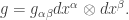
In modern cosmology, one can introduce on the spacetime (V,\mathbf g) a real scalar field \boldsymbol \psi with potential U as a smooth function of \boldsymbol\psi. A particular Einstein field theory is specified by the choice of an action principle with

\displaystyle\mathcal{L}_\mathrm{M}=-\frac{1}{2}|\nabla\boldsymbol\psi|^2_{\mathbf g}-U(\boldsymbol\psi).

To find its associated stress-energy tensor, we first look at \frac{{\delta {\mathcal{L}_{\text{M}}}}}{{\delta {g^{\mu \nu }}}}. Since the term U(\boldsymbol\psi) does not depend on the metric, we get

\displaystyle\frac{{\delta {\mathcal{L}_{\text{M}}}}}{{\delta {\mathbf g^{\mu \nu }}}} = \frac{1}{{\delta {\mathbf g^{\mu \nu }}}}\left( { - \frac{1}{2}(\delta {\mathbf g^{\mu \nu }}){\partial _{\mu }}\boldsymbol\psi {\partial _\nu }\boldsymbol\psi } \right) = - \frac{1}{2}{\partial _{\mu }}\boldsymbol\psi {\partial _\nu }\boldsymbol\psi,

(more…)

December 31, 2012

n+1 decomposition of the spacetime metric

Filed under: Uncategorized — Tags: — Ngô Quốc Anh @ 17:29

Let us introduce the components \gamma_{ij} of the n-metric \gamma of the hypersurface M with respect to the coordinates (x^i)

\displaystyle \gamma=\gamma_{ij}dx^i\otimes dx^j.

From the definition of the shift vector \beta, we can write

\displaystyle \beta_i=\gamma_{ij}\beta^j.

For the spacetime metric g of V, with respect to the coordinates (x^\alpha) we can also write

\displaystyle g=g_{\alpha\beta}dx^\alpha\otimes dx^\beta.

Keep in mind that \gamma=g|_M. Thanks to \partial_t = Nn+\beta, we obtain

\displaystyle \begin{array} {lcl}{g_{00}} &=&\displaystyle g({\partial _t},{\partial _t}) \hfill \\&=&\displaystyle g(Nn + \beta ,Nn + \beta ) \hfill \\ &=&\displaystyle {N^2}g(n,n) + g(\beta ,\beta ) \hfill \\ &=&\displaystyle - {N^2} + \gamma (\beta ,\beta ) \hfill \\ &=&\displaystyle - {N^2} + {\beta _i}{\beta ^i}. \hfill \\ \end{array}

Similarly, one can also obtain

\displaystyle\begin{array}{lcl} {g_{0i}} &=&\displaystyle g({\partial _t},{\partial _i}) \hfill \\&=&\displaystyle g(Nn + \beta ,{\partial _i}) \hfill \\&=&\displaystyle g({\beta _j}d{x^j},{\partial _i}) \hfill \\&=&\displaystyle {\beta _i}. \hfill \\ \end{array}

Finally, it is easy to see that

\displaystyle {g_{ij}} = g({\partial _i},{\partial _j}) = \gamma ({\partial _i},{\partial _j}) = {\gamma _{ij}}

for all i,j \geqslant 1.

(more…)

December 26, 2012

The evolution equations for the constraint equations

Filed under: Uncategorized — Tags: — Ngô Quốc Anh @ 1:12

Let us first recall the Gauss equation which is given by

\displaystyle\displaystyle\left\langle {\overline R (X,Y)Z,W} \right\rangle = \left\langle {R\left( {X,Y)Z} \right),W} \right\rangle - \left\langle {\mathrm{I\!I}(X,Z)} , {\mathrm{I\!I}(Y,W)} \right\rangle + \left\langle {\mathrm{I\!I}(Y,Z)} , {\mathrm{I\!I}(X,W)} \right\rangle.

This can be proved as the following

\displaystyle\begin{array}{lcl} R\left( {X,Y)Z} \right) &=&\displaystyle {\nabla _X}{\nabla _Y}Z - {\nabla _Y}{\nabla _X}Z - {\nabla _{[X,Y]}}Z \hfill \\&=& {\nabla _X}({\overline \nabla _Y}Z - \mathrm{I\!I}(Y,Z)) - {\nabla _Y}({\overline \nabla _X}Z - \mathrm{I\!I}(X,Z)) - ({\overline \nabla _{[X,Y]}}Z - \mathrm{I\!I}([X,Y],Z)) \hfill \\&=& {\nabla _X}({\overline \nabla _Y}Z) - {\nabla _X}(\mathrm{I\!I}(Y,Z)) - {\nabla _Y}({\overline \nabla _X}Z) + {\nabla _Y}(\mathrm{I\!I}(X,Z)) - {\overline \nabla _{[X,Y]}}Z + \mathrm{I\!I}([X,Y],Z) \hfill \\&=& {\overline \nabla _X}{\overline \nabla _Y}Z - \mathrm{I\!I}(X,{\overline \nabla _Y}Z) - {\overline \nabla _Y}{\overline \nabla _X}Z + \mathrm{I\!I}(Y,{\overline \nabla _X}Z) - {\nabla _X}(\mathrm{I\!I}(Y,Z)) + {\nabla _Y}(\mathrm{I\!I}(X,Z)) \hfill \\ &&- {\overline \nabla _{[X,Y]}}Z + \mathrm{I\!I}([X,Y],Z) \hfill \\&=&\overline R (X,Y)Z - \mathrm{I\!I}(X,{\overline \nabla _Y}Z) + \mathrm{I\!I}(Y,{\overline \nabla _X}Z) - {\nabla _X}(\mathrm{I\!I}(Y,Z)) + {\nabla _Y}(\mathrm{I\!I}(X,Z)) + \mathrm{I\!I}([X,Y],Z),\hfill \\ \end{array}

which implies

\displaystyle\begin{array}{lcl}\left\langle {\overline R (X,Y)Z,W} \right\rangle &=& \left\langle {R(X,Y)Z,W} \right\rangle + \left\langle {{\nabla _X}(\mathrm{I\!I}(Y,Z)),W} \right\rangle - \left\langle {{\nabla _Y}(\mathrm{I\!I}(X,Z)),W} \right\rangle \hfill \\&=& \left\langle {R(X,Y)Z,W} \right\rangle + \left\langle {{\nabla _X}(\mathrm{I\!I}(Y,Z)),W} \right\rangle - \left\langle {{\nabla _Y}(\mathrm{I\!I}(X,Z)),W} \right\rangle \hfill \\ &=& \left\langle {R(X,Y)Z,W} \right\rangle - \left\langle {\mathrm{I\!I}(Y,Z),{\nabla _X}W} \right\rangle + \left\langle {\mathrm{I\!I}(X,Z),{\nabla _Y}W} \right\rangle. \hfill \\ \end{array}

By using {\nabla _X}W = {\overline \nabla _X}W - \mathrm{I\!I}(X,W) and {\nabla _Y}W = {\overline \nabla _Y}W - \mathrm{I\!I}(Y,W), we finally obtain

\displaystyle\left\langle {\overline R (X,Y)Z,W} \right\rangle = \left\langle {R(X,Y)Z,W} \right\rangle + \left\langle {\mathrm{I\!I}(Y,Z),\mathrm{I\!I}(X,W)} \right\rangle - \left\langle {\mathrm{I\!I}(X,Z),\mathrm{I\!I}(Y,W)} \right\rangle

as claimed.

This identity is slightly different from that of the usual one since \langle n, n \rangle = -1 plays a crucial role in the above computation.

We denote by K_{\alpha\beta} the components of the scalar second fundamental form K, i.e.,

\displaystyle \mathrm{I\!I}(\cdot, \cdot) = -K(\cdot, \cdot) n.

(more…)

December 25, 2012

The Ricci equation

Filed under: Uncategorized — Tags: — Ngô Quốc Anh @ 2:58

Let us consider the Ricci identity defining the Riemann tensor R as measuring the lack of commutation of two successive covariant derivatives with respect to the connection \nabla associated with V‘s metric g

\nabla_\nu\nabla_\sigma w^\mu- \nabla_\sigma\nabla_\nu w^\mu=R_{\rho\nu\sigma}^\mu w^\rho.

By using w as the normal vector n, we find that

\nabla_\nu\nabla_\sigma n^\mu- \nabla_\sigma\nabla_\nu n^\mu=R_{\rho\nu\sigma}^\mu n^\rho.

We now project this tensor twice onto M, here the indices \mu and \nu, and once along n, here the index \sigma. Using the previous topic, we find that

\displaystyle {\gamma _{\alpha \mu }}{n^\sigma }\gamma _\beta ^\nu ({\nabla _\nu }{\nabla _\sigma }{n^\mu } - {\nabla _\sigma }{\nabla _\nu }{n^\mu }) = {\gamma _{\alpha \mu }}{n^\sigma }\gamma _\beta ^\nu R_{\rho \nu \sigma }^\mu {n^\rho }.

We now denote by a the following vector \nabla_n n. It is clear that a is a tangent vector.

This is clear since

\displaystyle n\cdot a = n \cdot \nabla_n n = \frac{1}{2}\nabla_n (n \cdot n)=0.

By extending the second fundamental K on M given by K(u,v)=- u \cdot \nabla_v n onto V, we find that K(u,v)=- u \cdot \nabla_v n - (a \cdot u)(n \cdot v) for all vectors u, v \in T_p(M).

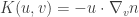
Again, this is clear since

\displaystyle \begin{gathered} K(u,v)\mathop = \limits^{\rm def} - (u + (n \cdot u)n) \cdot {\nabla _{v + (n \cdot v)n}}n \hfill \\ \qquad\quad\,\,= - (u + (n \cdot u)n) \cdot ({\nabla _v}n + (n \cdot v){\nabla _n}n) \hfill\\ \qquad\quad\,\,= - u \cdot {\nabla _v}n - (n \cdot v)u \cdot \underbrace {{\nabla _n}n}_a - (n \cdot u)\underbrace {n \cdot {\nabla _v}n}_0 - (n \cdot u)(n \cdot v)\underbrace {n \cdot {\nabla _n}n}_0 \hfill \\ \qquad\quad\,\,= - u \cdot {\nabla _v}n - (a \cdot u)(n \cdot v). \hfill \\ \end{gathered}

Thus, in components, we have

(more…)

December 19, 2012

How to decompose tensors into a purely spatial part and a timelike part?

Filed under: Riemannian geometry — Tags: — Ngô Quốc Anh @ 15:02

Today, we aim to talk about how to decompose tensors into a purely spatial part which lies in the hypersurfaces M and a timelike part which is normal to the spatial surface M?

Let us recall that M (called spatial surface) is a hypersurface of V (called the spacetime) of the dimension n+1. At each point p\in M, the space of all spacetime vectors can be orthogonally decomposed as

\displaystyle T_p(V)=T_p(M) \oplus \text{span}(n),

where \text{span}(n) stands for the 1-dimensional subspace of T_p(V) generated by the unit normal vector n to the surface M.

To do so, we need two projection operators.

The orthogonal projector onto M. In the literature, there exists such an operator, denoted by the symbol \gamma, given by

\displaystyle \begin{gathered} \gamma :{T_p}(V) \to {T_p}(M) \hfill \\ \qquad \quad\,\,\,v \mapsto v + (n \cdot v)n. \hfill \\ \end{gathered}

According to the above decomposition and thanks to

\displaystyle g_V = g_M + n \otimes n

with respect to any basis (e_i) of the space T_p(V), we have

\displaystyle \gamma_{ij}=g_{ij}+n_in_j,

which, by raising indices, gives

\displaystyle \gamma^i_{j}=\delta^i_{j}+n^in_j.

(more…)

December 10, 2012

Construction of spacetimes via solutions of the vacuum Einstein constraint equations and the propagation of the gauge condition

Filed under: Riemannian geometry — Tags: — Ngô Quốc Anh @ 23:10

A couple of days ago, we showed that the Einstein equations are essentially hyperbolic under the harmonic gauge. To be precise, the solvability of the equations

\displaystyle {\overline {{\text{Ric}}}} - \frac{1}{2}\overline g \text{Scal}_{\overline g} +\Lambda \overline g = \kappa\overline T,

is equivalent to solving the following hyperbolic system

\displaystyle - \frac{1}{2}{\overline g ^{km}}{\overline g _{ij,km}} = \Psi_{ij}((\overline g_{pq})_{0\leqslant p,q \leqslant n},(\overline g_{pq,r})_{0\leqslant p,q,r \leqslant n}),

provided \displaystyle {\lambda ^\alpha } = 0 for all \alpha = \overline {0,n} . Later on, when we consider the Cauchy problem for the Einstein equations on some appropriate framework, the first and second fundamental forms need to verify some constraint equations, [here and here].

By tracing the above equation, we obtain

\displaystyle \text{Scal}_{\overline g} + \frac{2n}{2 - n}\Lambda = \frac{2\kappa}{2 - n}\text{trace}_{\overline g}(\overline T),

which helps us to write

\displaystyle\overline {{\text{Ric}}} = \kappa \left( {\overline T - \frac{\overline g}{{n - 2}}{\text{trace}}_{\overline g}(\overline T )} \right) + \frac{2}{{n - 2}}\Lambda \overline g.

In the vacuum case, the above equation is nothing but

\displaystyle {\overline {{\text{Ric}}}}=\frac{2}{{n - 2}}\Lambda \overline g.

(more…)

December 8, 2012

Derivation of the Einstein constraint equations: The momentum constraint

Filed under: Riemannian geometry — Tags: — Ngô Quốc Anh @ 3:28

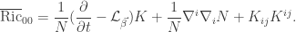
This entry is a continuation of the previous entry where we showed in detail the derivation of the Hamiltonian constrain in general relativity. Today, we derive the so-called momentum constraint equation.

First, let us recall the Codazzi equation which is given by the following identity

\displaystyle {R^ \bot }(X,Y)Z = ({\nabla _X}\mathrm{I\!I})(Y,Z) - ({\nabla _Y}\mathrm{I\!I})(X,Z).

Sometimes, we call it the Codazzi–Mainardi equation or the Ricci identity, which expresses the curvature of the normal bundle in terms of the second fundamental form. Using this, we obtain

\displaystyle\sum\limits_{i = 1}^n {{R^ \bot }({e_i},Y){e_i}} = \sum\limits_{i = 1}^n {({\nabla _{{e_i}}}\mathrm{I\!I})(Y,{e_i})} - \sum\limits_{i = 1}^n {({\nabla _Y}\mathrm{I\!I})({e_i},{e_i})}

for any tangent vector Y. Since R(e_i,Y)e_i, for all i \geqslant 1, belongs to the tangent space, there hold

\displaystyle\left\langle {R({e_i},Y){e_i},{e_0}} \right\rangle = 0 \quad \forall i = \overline{1,n}

and thus we can write

\displaystyle\left\langle {{R^ \bot }({e_i},Y){e_i},{e_0}} \right\rangle = \left\langle {R({e_i},Y){e_i},{e_0}} \right\rangle\quad \forall i = \overline{1,n}.

Moreover, by the antisymmetric property of the Riemann curvature tensor, i.e., R_{ijkl}=-R_{ijlk}, we know that

\displaystyle\left\langle {R({e_0},{e_i}){e_0},{e_0}} \right\rangle = 0\quad \forall i = \overline{1,n}

which immediately implies

(more…)

December 7, 2012

Derivation of the Einstein constraint equations: The Hamitonian constraint

Filed under: Riemannian geometry — Tags: — Ngô Quốc Anh @ 16:41

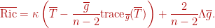
This entry is devoted to a derivation of the Einstein constraint equations. In fact, this is an expanded version of the previous entry. For the sake of simplicity, here we only derive the Hamiltonian constant equation. The momentum constaint equation will be considered in the coming entry.

Before we start, let us recall the following form of the Einstein equation with the cosmological constant \Lambda, that is

\displaystyle \text{Ric}_{\overline g}-\frac{1}{2}\overline g \text{Scal}_{\overline g}+\Lambda\overline g = \kappa T

where \kappa is a constant. The above equation is understood over the Lorentzian manifold (V,\overline g) of the dimension n+1. We shall use \langle\cdot, \cdot\rangle to denote \overline g(\cdot, \cdot).

Let us take (M,g) a submanifold of V of the dimension n. It is well-known that the Levi-Civita connection \nabla verifies the following decomposition

\displaystyle\overline\nabla_X Y=\nabla_X Y + \mathrm{I\!I}(X,Y)

for any smooth vector fields X and Y tangent to M and \mathrm{I\!I} is the second fundamental form.

We now mention the so-called Gauss equation. Before we do that, let us recall the Riemann curvature tensor R given by

\displaystyle R(X,Y)Z = \nabla_X\nabla_Y Z-\nabla_Y\nabla_X Z - \nabla_{[X,Y]}Z.

Furthermore, there holds

\displaystyle\nabla_X Y = \top(\overline\nabla_X Y),\quad \mathrm{I\!I}(X,Y) = \bot(\overline\nabla_X Y).

Then the Gauss equation is given by

\displaystyle\left\langle {\overline R (X,Y)Z,W} \right\rangle = \left\langle {R\left( {X,Y)Z} \right),W} \right\rangle + \left\langle {\mathrm{I\!I}(X,Z)} , {\mathrm{I\!I}(Y,W)} \right\rangle - \left\langle {\mathrm{I\!I}(Y,Z)} , {\mathrm{I\!I}(X,W)} \right\rangle.

We now let e_1,...,e_n be a local orthonormal frame field for M. Using the Gauss equation, we arrive at

\displaystyle\left\langle {\overline R \left( {{e_i},{e_j}} \right){e_i},{e_j}} \right\rangle = \left\langle {R({e_i},{e_j}){e_i},{e_j}} \right\rangle + \left\langle {\mathrm{I\!I}({e_i},{e_i})} ,{\mathrm{I\!I}({e_j},{e_j})} \right\rangle - \left\langle {\mathrm{I\!I}({e_i},{e_j})}, {\mathrm{I\!I}({e_i},{e_j})} \right\rangle,

(more…)

December 5, 2012

Why do the Einsteins equations describe the propagation of wavelike phenomena?

Filed under: PDEs, Riemannian geometry — Tags: — Ngô Quốc Anh @ 6:20

In order to formulate the initial value problem for the Einstein equations as nonlinear wave equations, we express the Einstein equations in terms of a partial di erential equation along with a gauge condition.

We suppose that (V,\overline g) is a Lorentzian manifold of the dimension n+1. The dummy indices will be from 0 up to n. In a coordinate system that will be fixed from now on, we have

\displaystyle\overline \Gamma _{ij}^k = \frac{1}{2}{\overline g ^{km}}({\overline g _{im,j}} + {\overline g _{jm,i}} - {\overline g _{ij,m}})

as Christoffel symbols for the metric \overline g.

By lower order terms we mean terms consisting of either no derivative or first order derivative of the metric \overline g. As such, terms consisting of derivatives of order higher than two will be called high order terms.

Let us now introduce the following notation

\displaystyle {\lambda ^\alpha } = {\square _{\overline g }}{x^\alpha } = {\overline g ^{ij}}x_{.ij}^\alpha = {\overline g ^{ij}}( - \overline \Gamma _{ij}^kx_{.k}^\alpha ) = - {\overline g ^{ij}}\overline \Gamma _{ij}^\alpha .

It is obvious to see that

\displaystyle - ({\overline g _{\alpha i}}\lambda _{,j}^\alpha + {\overline g _{\alpha j}}\lambda _{,i}^\alpha ) = {\overline g _{\alpha i}}{\overline g ^{km}}\overline \Gamma _{km,j}^\alpha + {\overline g _{\alpha j}}{\overline g ^{km}}\overline \Gamma _{km,i}^\alpha .

Since

\displaystyle\overline \Gamma _{km,j}^\alpha = \frac{1}{2}{\overline g ^{\alpha p}}({\overline g _{kp,mj}} + {\overline g _{mp,kj}} - {\overline g _{km,pj}}) + \text{lower order terms}

and

\displaystyle\overline \Gamma _{km,i}^\alpha = \frac{1}{2}{\overline g ^{\alpha q}}({\overline g _{kq,mi}} + {\overline g _{mq,ki}} - {\overline g _{km,qi}}) + \text{lower order terms},

(more…)

Older Posts »

Blog at WordPress.com.