Ngô Quốc Anh

June 28, 2010

A non-existence result for PDE Delta u=exp(u) in R^2

Filed under: PDEs — Tags: — Ngô Quốc Anh @ 0:28

We provide a proof of the following well known fact.

Theorem. There is no C^2 solution to

\displaystyle\begin{cases}\Delta u =e^u, & {\rm in } \, \mathbb R^2,\\\displaystyle\int_{\mathbb R^2}e^u<\infty.\end{cases}

I found this proof in a paper due to Y.Y. Li published in Commun. Math. Phys. in 1999 [here]. Before deriving the proof, let us recall the following notation known as the sphere mean in the literature. In \mathbb R^n we denote the integral

\displaystyle\displaystyle\frac{1}{\omega _n}{r^{n - 1}}\int_{\partial B\left( {0,r} \right)} {f\left( x \right)dS_x}

by \overline f(r). We call \overline f the average of f on the sphere S(0,r) of radius r, or sphere mean of a function around the origin. In this context, we simply have

\displaystyle\displaystyle\frac{1}{2\pi r}\int_{\partial B\left( {0,r} \right)} {f\left( x \right)dS_x}.

(more…)

June 25, 2010

Some operations on the Hölder continuous functions

Filed under: Giải Tích 1 — Tags: — Ngô Quốc Anh @ 4:37

This entry devotes the following fundamental question: if u is Hölder continuous, then how about u^\gamma for some constant \gamma? Throughout this entry, we work on \Omega \subset \mathbb R^n which is not necessarily bounded.

Firstly, we have an elementary result

Proposition. If f and g are \alpha-Hölder continuous and bounded, so is fg.

Proof. The proof is simple, we just observe that

\displaystyle\left| {f(x)g(x) - f(y)g(y)} \right| \leqslant \left| {f(x) - f(y)} \right||g(x)| + \left| {g(x) - g(y)} \right||f(y)|

which yields

\displaystyle\frac{{\left| {f(x)g(x) - f(y)g(y)} \right|}}{{{{\left| {x - y} \right|}^\alpha }}} \leqslant \frac{{\left| {f(x) - f(y)} \right|}}{{{{\left| {x - y} \right|}^\alpha }}}\left( {\mathop {\sup }\limits_\Omega |g(x)|} \right) + \frac{{\left| {g(x) - g(y)} \right|}}{{{{\left| {x - y} \right|}^\alpha }}}\left( {\mathop {\sup }\limits_\Omega |f(y)|} \right).

Consequently,

for any positive integer number n and any \alpha-Hölder continuous and bounded function u, function u^n is also \alpha-Hölder continuous and bounded.

Let us assume , u is \alpha-Hölder continuous and bounded, \gamma>0 is a constant. Let n =\left\lfloor \gamma \right\rfloor. Since \gamma \in \mathbb R, we may assume u is also bounded away from zero, that means there exist two constants 0<m<M<\infty such that

m<u(x)<M \quad \forall x \in \Omega.

We now study the \alpha-Hölder continuity of u^\gamma. Observe that function

\displaystyle f(t) = {t^{\left\lceil \gamma \right\rceil }}, \quad t>0

is sub-additive in the sense that

\displaystyle f(t_1+t_2) \leqslant f(t_1)+f(t_2), \quad \forall t_1,t_2>0.

(more…)

June 19, 2010

Existence of global super-solutions of the Lichnerowicz equations

Filed under: PDEs — Tags: , — Ngô Quốc Anh @ 19:16

This entry devotes the existence of global super-solutions to the Lichnerowicz equations in the study of the Einstein equations in general relativity. This terminology plays an important role in the study of non-CMC case of the Einstein equations in vacuum case.

This terminology first introduced in 2009 by a paper due to  M. Holst, G. Nagy and G. Tsogtgerel published in Comm. Math. Phys. [here]. In that paper, the solvability comes from the existence of both global sub- and global super-solutions together with some new fixed-point arguments which we have already discussed before [here]. Maxwell recently got a significant result by relaxing the existence of global sub-solutions [here] so that the existence of global super-solutions is enough to guarantee the solvability of the Einstein equations in non-CMC case.

In the vacuum case, the classification depends on the sign of the Yamabe invariants.

In the conformal method, in three dimensions the study of the Einstein equations becomes the study of existence of solution (\varphi, W) to a coupled system:

\displaystyle -8\Delta \varphi + R\varphi=-\frac{2}{3}\tau^2\varphi^5+|\sigma+\mathbb LW|^2\varphi^{-7}

and

\displaystyle {\rm div} \mathbb LW=\frac{2}{3}\varphi^6d\tau.

The first equation is usually called the Lichnerowicz equation

\displaystyle -8\Delta \varphi + R\varphi=-\frac{2}{3}\tau^2\varphi^5+|\beta|^2\varphi^{-7}

where \beta is a symmetric (0,2)-tensor.

Definition. We say \varphi_+ is a super-solution of the Lichnerowicz equation if

\displaystyle -8\Delta \varphi + R\varphi=-\frac{2}{3}\tau^2\varphi^5+|\beta|^2\varphi^{-7}.

Now we have

Definition. We say \varphi_+ is a global super-solution of the Lichnerowicz equation if whenever

0<\varphi \leqslant \varphi_+

then

\displaystyle -8\Delta \varphi + R\varphi=-\frac{2}{3}\tau^2\varphi^5+|\sigma+\mathbb LW_\varphi|^2\varphi^{-7}

where W_\varphi is a solution of second equation obtained from \varphi.

We are now in a position to derive main results.

(more…)

June 16, 2010

De Giorgi’s class and De Giorgi’s theorem

Filed under: PDEs — Tags: — Ngô Quốc Anh @ 18:55

In this entry, we introduce that De Giorgi’s class DG(\Omega) and prove that functions in DG(\Omega) are Holder continuous. This has as a consequence the celebrated De Giorgi’s theorem saying that solutions of second-order elliptic equations with bounded measurable coefficients are Holder continuous.

Let us study H^1-solutions of

\displaystyle\int_\Omega {{A^{\alpha \beta }}(x){\nabla _\alpha }u{\nabla _\beta }\varphi dx} = 0, \quad \varphi \in H_0^1(\Omega )

where A is assumed to be of class L^\infty(\Omega). Our aim is to show that u is in fact Holder continuous. The key idea is to use the Cacciopoli inequality on level sets of u.

Definition (De Giorgi’s class). We define the De Giorgi’s class (DG(\Omega)) to consist of all u \in H^1(\Omega) which satisfy

\displaystyle \int_{{B_\rho }} {{{\left| {\nabla {{(u - k)}^ + }} \right|}^2}dx} \leqslant \frac{c}{{{{(R - \rho )}^2}}}\int_{{B_R}} {{{\left| {{{(u - k)}^ + }} \right|}^2}dx} , \quad \forall k \in \mathbb{R}.

The following remark is useful.

  1. If u is a sub-solution then u \in DG(\Omega).
  2. If u is a super-solution then -u \in DG(\Omega).
  3. If u \in DG(\Omega) then u+{\rm const} \in DG(\Omega).
  4. In the definition of the De Giorgi class, exponent p=2 can be replaced by any p>1.

If we denote by A the level set of u, that is

A(k,r)=\{x \in B_r : u(x)>k\}

then if u \in DG(\Omega) by choosing a cut-off function

\displaystyle \eta \in C_0^\infty\left(B_\frac{R+\rho}{2}\right), \quad \eta \equiv 1, \quad {\rm on } B_\rho

(more…)

June 13, 2010

Achieving regularity results via bootstrap argument, 2

Filed under: PDEs — Tags: , — Ngô Quốc Anh @ 1:37

Today, we shall discuss a very strong tool in the theory of elliptic PDEs in order to achieve the smoothness of solution. The tool we just mentioned is known as the Calderón-Zygmund L^p estimates or the Calderón-Zygmund inequality. Precisely,

Theorem (Calderón-Zygmund). Let 1<p<\infty and f \in L^p(\Omega) (\Omega is open and bounded). Let u be the weak solution of the following PDE

\displaystyle \Delta u = f.

Then u\in W^{2,p}(\Omega') for any \Omega' \Subset \Omega.

Let us consider the regularity of solution of

\displaystyle \Delta u +\Gamma(u)|\nabla u|^2=0

with a smooth \Gamma. We also require that \Gamma is bounded.

Motivation. The above PDE occurs as the Euler-Lagrange equation of the variational problem

\displaystyle I(u)=\int_\Omega g(u(x))|\nabla u(x)|^2dx \to {\rm min}

with a smooth g with is bounded and bounded away from zero. Moreover, g' is bounded.

In fact, to derive the Euler-Lagrange equation, we consider

\displaystyle I(u + t\varphi ) = \int_\Omega {g(u + t\varphi ){{\left| {\nabla (u + t\varphi )} \right|}^2}dx}

where \varphi \in H_0^{1,2}(\Omega). In that case

\displaystyle \frac{d}{{dt}}I(u + t\varphi ) = \int_\Omega {\left[ { - 2g(u)\Delta u - g'(u){{\left| {\nabla u} \right|}^2}} \right]\varphi dx}

after integrating by parts and assuming for the moment u \in C^2. Thus, the minimizer will verify

\displaystyle - 2g(u)\Delta u - g'(u){\left| {\nabla u} \right|^2} = 0

(more…)

June 11, 2010

The method of moving planes: Elliptic systems in the whole space

Filed under: PDEs — Tags: — Ngô Quốc Anh @ 5:13

Li Ma and Baiyu Liu recently announced a new result accepted in Advances in Mathematics journal [here]. In that elegant paper, they considered the following system of equations

\displaystyle\left\{ \begin{gathered} - \Delta u = g(u,v), \hfill \\ - \Delta v = f(u,v), \hfill \\ u > 0,v > 0, \hfill \\ \end{gathered} \right.

in the whole space \mathbb R^n with n\geqslant 3 where f and g are two smooth functions in \mathbb R^2_+.

This work is closely related to works done in [here] and [here]. Precisely, in [here], the authors have proved that classical solution (u, v) of the PDEs is symmetric about some points x_1, x_2 \in \mathbb R^n respectively, under assumptions

  1. u(x) \to 0, v(x) \to 0 as |x| \to \infty;

  2. \displaystyle\frac{{\partial g}}{{\partial v}}(u,v) \geqslant 0, \quad \frac{{\partial f}}{{\partial u}} (u,v)\geqslant 0,\quad\forall (u,v) \in \left[ {0, + \infty } \right) \times \left[ {0, + \infty } \right);

  3. \displaystyle\frac{{\partial g}}{{\partial u}}(0,0) < 0, \quad \frac{{\partial f}}{{\partial v}}(0,0) < 0;

  4. \displaystyle\det \left( {\begin{array}{*{20}{c}} {\frac{{\partial g}}{{\partial u}}} & {\frac{{\partial g}}{{\partial v}}} \\ {\frac{{\partial f}}{{\partial u}}} & {\frac{{\partial f}}{{\partial v}}} \\ \end{array} } \right)(0,0) > 0.

In this paper, the authors relax the hypothesis (4), for the price of supposing exact growth of the solutions at infinity, and of the nonlinearities at zero. Precisely, they proved

Theorem. Let (u, v) be a classical solution of the system and f,g \in C^1([0,\infty) \times [0,\infty), \mathbb R). Suppose

  1. \displaystyle u(x) \sim \frac{1}{{{{\left| x \right|}^\alpha }}}, \quad v(x) \sim \frac{1}{{{{\left| x \right|}^\beta }}}, \quad \left| x \right| \to \infty;
  2. \displaystyle \frac{{\partial g}}{{\partial u}}\lesssim {u^{p - 1}},\quad\frac{{\partial f}}{{\partial v}} \lesssim {v^{q - 1}},\quad u \to {0^ + },\quad v \to {0^ + } ;
  3. \displaystyle \frac{{\partial g}}{{\partial v}}\lesssim {u^{a -  1}},\quad\frac{{\partial f}}{{\partial u}} \lesssim {v^{b - 1}},\quad u  \to {0^ + },\quad v \to {0^ + } ;
  4. \displaystyle \frac{{\partial g}}{{\partial v}} > 0,\quad\frac{{\partial f}}{{\partial u}} > 0,\quad\forall (u,v) \in (0,\infty ) \times (0,\infty );

where positive constants \alpha, \beta, p, q, a, b satisfy

\displaystyle\alpha (p - 1) > 2,\beta (q - 1) > 2,\alpha (a - 1) > 2,\beta (b - 1) > 2.

Then there exists a point in x_0 \in \mathbb R^n, such that

u(x)=u(|x-x_0|), \quad v(x)=v(|x-x_0|).

The proof used is the method of moving planes. This kind of system is also a generalization of the Lane-Emden system given by

\displaystyle\left\{ \begin{gathered} - \Delta u = {v^b }, \hfill \\ - \Delta v = {u^a }. \hfill \\ \end{gathered} \right.

It can also be applied to the following system

\displaystyle\left\{ \begin{gathered} - \Delta u = - {u^p} + {v^b}, \hfill \\ - \Delta v = {u^a} - {v^q}. \hfill \\ \end{gathered} \right.

However, it is no longer able to apply to

\displaystyle\left\{ \begin{gathered} - \Delta u = {u^p} - {v^b}, \hfill \\ - \Delta v = - {u^a} + {v^q}. \hfill \\ \end{gathered} \right.

In fact, hypothesis (4) plays an important role in their argument. To our knowledge, the latter case is still open.

June 9, 2010

Invariance under fractional linear transformations

Filed under: Giải Tích 5, Giải Tích 6 (MA5205) — Tags: — Ngô Quốc Anh @ 5:02

I just read the following result due to Loss-Sloane published in J. Funct. Anal. this year [here]. This is just a lemma in their paper that I found very interesting.

Let f be any function in C_0^\infty(\mathbb R \setminus \{0\}). Consider the inversion x \mapsto \frac{1}{x} and set

\displaystyle g(x) = {\left| x \right|^{\alpha - 1}}f\left( {\frac{1}{x}} \right).

Then g \in C_0^\infty(\mathbb R) and

\displaystyle\iint\limits_{{\mathbb{R}^2}} {\frac{{{{\left| {g(x) - g(y)} \right|}^2}}}{{{{\left| {x - y} \right|}^{\alpha + 1}}}}dxdy} = \iint\limits_{{\mathbb{R}^2}} {\frac{{{{\left| {f(x) - f(y)} \right|}^2}}}{{{{\left| {x - y} \right|}^{\alpha + 1}}}}dxdy}.

Proof. For fixed \varepsilon consider the regions

\displaystyle {R_1}: = \left\{ {(x,y) \in {\mathbb{R}^2}:\left| {\frac{x}{y}} \right| > 1 + \varepsilon } \right\}

and likewise,

\displaystyle {R_2}: = \left\{ {(x,y) \in {\mathbb{R}^2}:\left|  {\frac{y}{x}} \right| > 1 + \varepsilon } \right\}.

(more…)

June 7, 2010

Some important functional inequalities, 2


This entry can be considered as a continued part to a recent entry where lots of significantly important inequalities (Hardy, Opial, Rellich, Serrin, Caffarelli–Kohn–Nirenberg, Gagliardo-Nirenberg-Sobolev, Horgan) have been considered.

Today we shall continue to list here more important inequalities in the literature. Given 1\leqq q < n, 0 < \theta \leqq 1, s>1, define the number r by

\displaystyle\frac{1}{s} - \frac{1}{r} = \theta \left( {\frac{1}{s} - \frac{1}{{{q^ \star }}}} \right)

where

\displaystyle q^\star=\frac{n-q}{nq}.

Gagliardo-Nirenberg’s inequality. For any u \in C_0^\infty(\mathbb R^n) one has

\displaystyle {\left( {\int_{{\mathbb{R}^n}} {|u{|^r}dx} } \right)^{\frac{1}{r}}} \leqq C{\left( {\int_{{\mathbb{R}^n}} {|\nabla u{|^q}dx} } \right)^{\frac{\theta }{q}}}{\left( {\int_{{\mathbb{R}^n}} {|u{|^s}dx} } \right)^{\frac{{1 - \theta }}{s}}}.

When \theta=1 and r=q^\star, Gagliardo-Nirenberg’s inequality then becomes the well-known Sobolev inequality.

Sobolev’s inequality. For any u \in C_0^\infty(\mathbb R^n) one has

\displaystyle {\left( {\int_{{\mathbb{R}^n}} {|u{|^{{q^ \star }}}dx} } \right)^{\frac{1}{{{q^ \star }}}}} \leqq K(n,q){\left( {\int_{{\mathbb{R}^n}} {|\nabla u{|^q}dx} } \right)^{\frac{1}{q}}}.

The best constant K(n,q) has been obtained by Aubin [here] and Talenti [here], independently. Namely, they showed that

\displaystyle K(n,1) = \frac{1}{n}\omega _n^{ - \frac{1}{n}}

and

\displaystyle K(n,q) = \frac{1}{n}{\left( {\frac{{n(q - 1)}}{{n - q}}} \right)^{\frac{{q - 1}}{q}}}{\left( {\frac{{\Gamma (n + 1)}}{{n{\omega _n}\Gamma \left( {\frac{n}{q}} \right)\Gamma \left( {n + 1 - \frac{n}{q}} \right)}}} \right)^{\frac{1}{n}}}, \quad q > 1

where \omega_n is the volume of the unit ball in \mathbb R^n and \Gamma the gamma function.

When \theta=\frac{n}{n+2}, q=2, and r=2, Gagliardo-Nirenberg’s inequality then becomes the well-known Nash inequality.

Nash’s inequality. For any u \in C_0^\infty(\mathbb R^n) one has

\displaystyle {\left( {\int_{{\mathbb{R}^n}} {|u{|^2}dx} } \right)^{1 + \frac{2}{n}}} \leqq C(n)\left( {\int_{{\mathbb{R}^n}} {|\nabla u{|^2}dx} } \right){\left( {\int_{{\mathbb{R}^n}} {|u|dx} } \right)^{\frac{4}{n}}}.

The best constant C(n) for the Nash inequality is given by

\displaystyle C(n) = \frac{{2{{\left( {\frac{{n + 2}}{2}} \right)}^{\frac{{n + 2}}{n}}}}}{{n\lambda _1^N\omega _n^{\frac{2}{n}}}}

where \lambda _1^N is the first non-zero Neumann eigenvalue of the Laplacian operator in the unit ball.  This come from a joint work between Carlen and Loss [here].

Another consequence of Gagliardo-Nirenberg’s inequality is the logarithmic Sobolev inequality.

logarithmic Sobolev’s inequality. For any u \in C_0^\infty(\mathbb R^n) one has

\displaystyle\int_{{\mathbb{R}^n}} {{u^2}{{(\log u)}^2}dx} \leqslant \frac{n}{2}\log \left( {\widetilde C\int_{{\mathbb{R}^n}} {|\nabla u{|^2}dx} } \right)

where u also satisfies

\displaystyle\int_{{\mathbb{R}^n}} {{u^2}dx} = 1.

In fact, it can be obtained as the limit case when \theta \to 0, that is, r=2 and s \to r, s<r. To see this, let us first notice the fact that the constant C in Gagliardo-Nirenberg’s inequality is independent of s. We can rewrite Gagliardo-Nirenberg’s inequality as
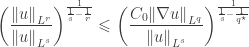
\displaystyle{\left( {\frac{{{{\left\| u \right\|}_{{L^r}}}}}{{{{\left\| u \right\|}_{{L^s}}}}}} \right)^{\frac{1}{{\frac{1}{s} - \frac{1}{r}}}}} \leqslant {\left( {\frac{{{C_0}{{\left\| {\nabla u} \right\|}_{{L^q}}}}}{{{{\left\| u \right\|}_{{L^s}}}}}} \right)^{\frac{1}{{\frac{1}{s} - \frac{1}{{{q^ \star }}}}}}}

where C_0=C^\frac{1}{\theta}. It then follows that

\displaystyle\frac{{\log {{\left\| u \right\|}_{{L^r}}} - {{\left\| u \right\|}_{{L^s}}}}}{{\frac{1}{s} - \frac{1}{r}}} \leqslant \frac{1}{{\frac{1}{s} - \frac{1}{{{q^ \star }}}}}\log \left( {{C_0}\frac{{{{\left\| {\nabla u} \right\|}_{{L^q}}}}}{{{{\left\| u \right\|}_{{L^s}}}}}} \right).

Thus when s \to r^- we get

\displaystyle\int_{{\mathbb{R}^n}} {\left[ {{u^r}\log {{\left( {\frac{u}{{{{\left\| u \right\|}_{{L^r}}}}}} \right)}^r}} \right]dx} \leqq \frac{1}{{\frac{1}{s} - \frac{1}{{{q^ \star }}}}}\left\| u \right\|_{{L^r}}^r\log \left( {{C_0}\frac{{{{\left\| {\nabla u} \right\|}_{{L^q}}}}}{{{{\left\| u \right\|}_{{L^r}}}}}} \right)

where we have used the fact that the function

\displaystyle\varphi (u) = \log {\left\| u \right\|_{{L^u}}}

satisfies

\displaystyle - \left\| u \right\|_{{L^r}}^r\varphi '\left( {\frac{1}{r}} \right) = \int_{{\mathbb{R}^n}} {\left[ {{u^r}\log {{\left( {\frac{u}{{{{\left\| u \right\|}_{{L^r}}}}}} \right)}^r}} \right]dx} .

Therefore, replacing r = q = 2 and writing \widetilde C = \sqrt{C_0}, we obtain the logarithmic Sobolev’s inequality.

The best constant for the logarithmic Sobolev inequality is given by

\displaystyle\widetilde C(n) = \frac{2}{{n\pi e}}.

We refer the reader to a book due to Hebey entitled “Nonlinear analysis on manifolds: Sobolev spaces and inequalities” for details.

The best constant for the Gagliardo-Nirenberg inequality is not completely solved. In some cases, we was able to find its best constants [here, here].

See also: Sobolev type inequalities on Riemannian manifolds

June 5, 2010

Why the conformal method is useful in studying the Einstein equations?

Filed under: Nghiên Cứu Khoa Học, PDEs, Riemannian geometry — Tags: — Ngô Quốc Anh @ 19:20

I presume you have some notions about general relativity, especially the Einstein equations

{\rm Eins}_{\alpha\beta}=T_{\alpha\beta}.

As these equations are basically hyperbolic for a suitable metric, it is reasonable to study the Cauchy problems for them. Under the Gauss and Codazzi conditions, we have two constraints called Hamiltonian and Momentum constrains. Cauchy problem is to determine the solvable of these constrains of variables K-the extrinsic curvature and g-the spatial metric. Interestingly, the conformal method says that we can start with an arbitrary metric then we recast the constrain equations into a form which is more amenable to analysis by splitting the Cauchy data. In this method, we try to solve \gamma within the conformal class represented by the initial metric. So, in general, the conformal factor is chosen so that we eventually have a simplest model.

This idea is given via the following theorem.

Theorem. Let \mathcal D =(\gamma, \sigma, \tau,\psi,\pi) be a conformal initial data set for the Einstein-scalar field constraint equations on \Sigma. If

\displaystyle \widetilde \gamma =\theta^\frac{4}{n-2}\gamma

for a smooth positive function \theta, then we define the corresponding conformally transformed initial data set by

\displaystyle\widetilde{\mathcal D} =(\widetilde\gamma, \widetilde \sigma, \widetilde \tau,\widetilde\psi,\widetilde \pi)=(\theta^\frac{4}{n-2}\gamma, \theta^{-2}\sigma, \tau,\psi,\theta^\frac{-2n}{n-2}\pi).

Let W be the solution to the conformal form of the momentum constrain equation w.r.t. the conformal initial data set \mathcal D and let \widetilde W be the solution to the conformal form of the momentum constrain equation w.r.t. the conformal initial data set \widetilde{\mathcal D} (we just assume both exist). Then \varphi is a solution to the Einstein scalar field Lichnerowicz equation for the conformal data \mathcal D with W

\displaystyle \Delta_\gamma \varphi - \mathcal R_{\gamma, \psi}\varphi +\mathcal A_{\gamma, W, \pi}\varphi^{-\frac{3n-2}{n-2}}-\mathcal B_{\tau, \psi}\varphi^\frac{n+2}{n-2}=0

if and only if \theta^{-1}\varphi is a solution to the Einstein scalar field Lichnerowicz equation for the conformal data \widetilde{\mathcal D} with \widetilde W

\displaystyle \Delta_{\widetilde\gamma} (\theta^{-1}\varphi) - \mathcal R_{\widetilde\gamma, \widetilde\psi}(\theta^{-1}\varphi) +\mathcal A_{\widetilde\gamma, \widetilde W, \widetilde\pi}(\theta^{-1}\varphi)^{-\frac{3n-2}{n-2}}-\mathcal B_{\widetilde\tau, \widetilde\psi}(\theta^{-1}\varphi)^\frac{n+2}{n-2}=0.

We refer the reader to a paper due to Yvonne Choquet-Bruhat et al. [here] published in Class. Quantum Grav. in 2007 for details. We adopt this theorem from that paper, however, there is no proof there.

(more…)

June 3, 2010

Lower bound for integral of exp(u)

Filed under: PDEs — Tags: — Ngô Quốc Anh @ 21:51

As mentioned before, today I will derive a very short and beautiful proof concerning the lower bound of \int\exp(u(x))dx where u, a positive solution to the following PDE

\displaystyle -\Delta u =e^{u(x)}, \quad x \in \mathbb R^2.

This proof I firstly learned from a paper published in Duke Math. J. in 1991 by W. Cheng and C. Li [here].

We assume

\displaystyle \int_{\mathbb R^2} e^{u(x)}dx < \infty.

Denote by \Omega_t the following set

\Omega_t = \{ x \in \mathbb R^2 : u(x)>t\}.

It follows from this topic that

\displaystyle \int_{\Omega_t} e^{u(x)}dx =-\int_{\Omega_t}\Delta u dx = \int_{\partial \Omega_t} |\nabla u|d\sigma.

Also, it follows from this topic that

\displaystyle -\frac{d}{dt}\int_{\Omega_t}dx =\int_{\partial \Omega_t} \frac{1}{|\nabla u|}d\sigma.

Thus, by the Schwarz inequality and the isoperimetric inequality

\displaystyle \left(\int_{\partial\Omega_t} \frac{1}{|\nabla u|}d\sigma\right)\left(\int_{\partial\Omega_t}|\nabla u| d\sigma\right) \geqslant |\partial\Omega_t|^2 \geqslant 4\pi |\Omega_t|.

Hence

\displaystyle -\left(\frac{d}{dt}\int_{\Omega_t}dx\right) \left(\int_{\Omega_t} e^{u(x)}dx\right)\geqslant 4\pi |\Omega_t|.

So

\displaystyle \frac{d}{dt}\left(\int_{\Omega_t} e^{u(x)}dx\right)^2=2\left(\int_{\Omega_t} e^{u(x)}dx\right)\frac{d}{dt}\left(\int_{\Omega_t} e^{u(x)}dx\right).

It is worth noticing that

\displaystyle\frac{d}{dt}\left(\int_{\Omega_t} e^{u(x)}dx\right)=e^t\frac{d}{dt}\left(\int_{\Omega_t}dx\right)

which yields

\displaystyle \frac{d}{dt}\left(\int_{\Omega_t} e^{u(x)}dx\right)^2=2\left(\int_{\Omega_t} e^{u(x)}dx\right)e^t\frac{d}{dt}\left(\int_{\Omega_t}dx\right) \leqslant -8\pi e^t\int_{\Omega_t}dx.

Integrating from -\infty to \infty gives

\displaystyle -\left(\int_{\mathbb R^2} e^{u(x)}dx\right)^2\leqslant -8\pi\int_{\mathbb R^2}e^{u(x)}dx

which implies

\displaystyle \int_{\mathbb R^2} e^{u(x)}dx \geqslant 8\pi.

Older Posts »

Create a free website or blog at WordPress.com.