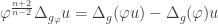
In this topic we consider the analysis of solutions of the following system entitled Toda system

Following is our main result
Lemma 1. The following identities
hold.
In this topic we consider the analysis of solutions of the following system entitled Toda system
Following is our main result
Lemma 1. The following identities
hold.
Let us consider the following integral in
when 
Obviously, the sphere 
so
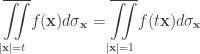
If we wish to work on the average, the formula is much simpler than that, precisely
that means
where the bar means the average.
More general, we get

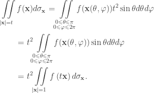
Today, we try to evaluate the following surface integral in 
Proposition. Let
be a continuous function. Then we have
here we denote
.
Proof. Remark that the integral only depends on 

where

This system of coordinates can be seen via the picture below

Let me provide another proof of Example 2 in this topic.
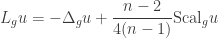
Example 2. The conformal Laplacian operator acting on a smooth function 
is conformal invariant.
The proof relies on the following fact
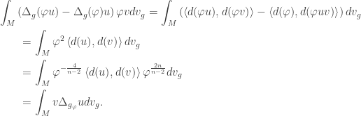
Proposition. Under a conformal change
, we have
where
and
are the volume elements with respect to metrics
and
respectively.
We are now in a position to prove example 2. For simplicity, let us consider the following conformal change 
Step 1. Showing
Proof. Indeed, for any test function 

We now use Laplace-de Rham operator for the sake of simplicity. Note that Laplace–de Rham operator is the Laplacian differential operator on sections of the bundle of differential forms on a pseudo-Riemannian manifold. However, the Laplace-de Rham operator is equivalent to the definition of the Laplace–Beltrami operator when acting on a scalar function. Precisely,

Therefore
Step 2. Showing the scalar curvature equation

Equivalently,
Step 3. Showing

Proof. Clearly
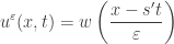
Let us consider a very simple class of schemes solving the convection equations entitled the upwind schemes. Precisely, let us consider
together with the following initial data

It is well-known that the above problem has a unique solution given by 

Since the upwind schemes are well-known and appear in most of numerical analysis’s textbooks, what I am trying to do here is to give some basic ideas together with their motivation.
First of all, the original upwind schemes are just explicit one-step schemes. Upwind schemes use an adaptive or solution-sensitive finite difference stencil to numerically simulate more properly the direction of propagation of information in a flow field. The upwind schemes attempt to discretize hyperbolic partial differential equations by using differencing biased in the direction determined by the sign of the characteristic speeds. Historically, the origin of upwind methods can be traced back to the work of Courant, Isaacson, and Reeves who proposed the CIR method.
Discretization. Like the finite difference methods, we need to use a a grid with points 

for some spatial grid size 


Let 


We start with the following terminology called “a conformal change“.
Definition. If
is another metric on
on
, then
is called a conformal change of Riemannian metric.
We are now in a position to define the so-called “conformal invariant operators“.
Definition. We call a metrically de fined operator
conformally covariant of bi-degree
if under the conformal change of metric
and
.
Example 1. The Laplace-Beltrami operator is conformal invariant.
Proof. Let us recall from this topic that on 
and in local coordinates it is given as follows

By a change of metric 

Indeed, in local coordinates
which implies

Besides,

Let us start with a given 
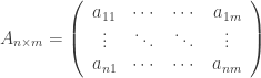
The aim of this entry is to compare nullspace, column space and row space between 


Nullspaces. We start with the following result
Proposition 1. The following
holds.
Proof. Pick an arbitrary element 

so

Conversely, assume 


Consequently,

In other words, 
Remark. 
Regarding to matrix

Similarly, involving matrix

It now follows from Proposition 1 that

In other words, column and row spaces associated to
Row spaces. We prove the following
Proposition 2. The following
holds.
Proof. The way to compare column spaces is to use the following facts
and
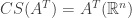
Equivalently, from the first fact we need to show that

In term of the second fact, once you have a suitable matrix 

which turns out to be
since they have the same dimension, equality occurs.
Remark. This comes from the proof above. If you have a good matrix

Column spaces. We prove the following
Proposition 3. The following
holds.
Proof. This is trivial by using Proposition 2.
Remark. If you have a good matrix 

In numerical analysis, the Bramble-Hilbert lemma, named after James H. Bramble and Stephen R. Hilbert, bounds the error of an approximation of a function 


Theorem. Over a sufficiently domain
, there exists a constant
such that
for every
where
and
denote the norm and semi-norm of the Sobolev space
.
This is similar to classical numerical analysis, where, for example, the error of linear interpolation
Additional assumptions on the domain are needed for the Bramble-Hilbert lemma to hold. Essentially, the boundary of the domain must be “reasonable”. For example, domains that have a spike or a slit with zero angle at the tip are excluded. Lipschitz domains are reasonable enough, which includes convex domains and domains with 
The main use of the Bramble-Hilbert lemma is to prove bounds on the error of interpolation of function
This entry deals with the conservation law
and the problem of determining which weak solutions of the above equation are to be considered acceptable. We shall use the idea of vanishing viscosity whereby one considers instead the equation
in the limit as 
We consider a jump discontinuity in the solution 


and the problem is to determine further conditions on the shock that will hopefully lead to uniqueness as well of existence of weak solutions to the initial value problem for the problem.
Traveling waves. One way to get an answer to our problem is to look for traveling wave solutions to our problem, i.e., solutions on the form
Substituting this into the equation gives

We can integrate this once to get

Now we get
and therefore we shall insist that

In particular, the right hand side of the above ODE has a limit as 


Clearly,

Besides, the above identity states that 


Theorem. The given equation admits a traveling wave solution of the form above satisfying
if and only if
for all
are chosen so that the above expression is zero when
or
.
O. Oleinik entropy condition. The entropy condition given by the above theorem is equivalent to the inequalities

This entropy condition was suggested by O. Oleinik but since she gave another entropy condition more commonly associated with her name this condition is often referred to as the viscous profile entropy condition.
Lax entropy condition. The Lax entropy condition is the pair of inequalities
in the case when
We now consider another kind of problem involving biharmonic operator. Let us assume 
in
Theorem. The following identity
holds.
![\displaystyle\begin{gathered} \left( {1 - \frac{n}{2}} \right)\int_{{B_r}(0)} {|\nabla {u_1}{|^2}dx} + r\left[ {\frac{1}{2}\int_{\partial {B_r}(0)} {|\nabla {u_1}{|^2}d\sigma } - \int_{\partial {B_r}(0)} {{{\left| {\frac{{\partial {u_1}}}{{\partial \nu }}} \right|}^2}d\sigma } } \right] \hfill \\ \qquad\qquad= - 2n\int_{{B_r}(0)} {{e^{{u_1}}}dx} + 2\int_{\partial {B_r}(0)} {r{e^{{u_1}}}dx} - \int_{{B_r}(0)} {{e^{{u_2}}}(x\cdot\nabla {u_1})dx} , \hfill \\ \left( {1 - \frac{n}{2}} \right)\int_{{B_r}(0)} {|\nabla {u_2}{|^2}dx} + r\left[ {\frac{1}{2}\int_{\partial {B_r}(0)} {|\nabla {u_2}{|^2}d\sigma } - \int_{\partial {B_r}(0)} {{{\left| {\frac{{\partial {u_2}}}{{\partial \nu }}} \right|}^2}d\sigma } } \right] \hfill \\ \qquad\qquad= - 2n\int_{{B_r}(0)} {{e^{{u_2}}}dx} + 2\int_{\partial {B_r}(0)} {r{e^{{u_2}}}dx} - \int_{{B_r}(0)} {{e^{{u_1}}}(x\cdot\nabla {u_2})dx} , \hfill \\ \end{gathered}](https://s0.wp.com/latex.php?latex=%5Cdisplaystyle%5Cbegin%7Bgathered%7D+%5Cleft%28+%7B1+-+%5Cfrac%7Bn%7D%7B2%7D%7D+%5Cright%29%5Cint_%7B%7BB_r%7D%280%29%7D+%7B%7C%5Cnabla+%7Bu_1%7D%7B%7C%5E2%7Ddx%7D+%2B+r%5Cleft%5B+%7B%5Cfrac%7B1%7D%7B2%7D%5Cint_%7B%5Cpartial+%7BB_r%7D%280%29%7D+%7B%7C%5Cnabla+%7Bu_1%7D%7B%7C%5E2%7Dd%5Csigma+%7D+-+%5Cint_%7B%5Cpartial+%7BB_r%7D%280%29%7D+%7B%7B%7B%5Cleft%7C+%7B%5Cfrac%7B%7B%5Cpartial+%7Bu_1%7D%7D%7D%7B%7B%5Cpartial+%5Cnu+%7D%7D%7D+%5Cright%7C%7D%5E2%7Dd%5Csigma+%7D+%7D+%5Cright%5D+%5Chfill+%5C%5C+%5Cqquad%5Cqquad%3D+-+2n%5Cint_%7B%7BB_r%7D%280%29%7D+%7B%7Be%5E%7B%7Bu_1%7D%7D%7Ddx%7D+%2B+2%5Cint_%7B%5Cpartial+%7BB_r%7D%280%29%7D+%7Br%7Be%5E%7B%7Bu_1%7D%7D%7Ddx%7D+-+%5Cint_%7B%7BB_r%7D%280%29%7D+%7B%7Be%5E%7B%7Bu_2%7D%7D%7D%28x%5Ccdot%5Cnabla+%7Bu_1%7D%29dx%7D+%2C+%5Chfill+%5C%5C+%5Cleft%28+%7B1+-+%5Cfrac%7Bn%7D%7B2%7D%7D+%5Cright%29%5Cint_%7B%7BB_r%7D%280%29%7D+%7B%7C%5Cnabla+%7Bu_2%7D%7B%7C%5E2%7Ddx%7D+%2B+r%5Cleft%5B+%7B%5Cfrac%7B1%7D%7B2%7D%5Cint_%7B%5Cpartial+%7BB_r%7D%280%29%7D+%7B%7C%5Cnabla+%7Bu_2%7D%7B%7C%5E2%7Dd%5Csigma+%7D+-+%5Cint_%7B%5Cpartial+%7BB_r%7D%280%29%7D+%7B%7B%7B%5Cleft%7C+%7B%5Cfrac%7B%7B%5Cpartial+%7Bu_2%7D%7D%7D%7B%7B%5Cpartial+%5Cnu+%7D%7D%7D+%5Cright%7C%7D%5E2%7Dd%5Csigma+%7D+%7D+%5Cright%5D+%5Chfill+%5C%5C+%5Cqquad%5Cqquad%3D+-+2n%5Cint_%7B%7BB_r%7D%280%29%7D+%7B%7Be%5E%7B%7Bu_2%7D%7D%7Ddx%7D+%2B+2%5Cint_%7B%5Cpartial+%7BB_r%7D%280%29%7D+%7Br%7Be%5E%7B%7Bu_2%7D%7D%7Ddx%7D+-+%5Cint_%7B%7BB_r%7D%280%29%7D+%7B%7Be%5E%7B%7Bu_1%7D%7D%7D%28x%5Ccdot%5Cnabla+%7Bu_2%7D%29dx%7D+%2C+%5Chfill+%5C%5C+%5Cend%7Bgathered%7D&bg=ffffff&fg=333333&s=0&c=20201002)


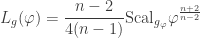
![\displaystyle\begin{gathered} {L_g}(\varphi u) = - {\Delta _g}(\varphi u) + \frac{{n - 2}}{{4(n - 1)}}{\rm Scal}_g\varphi u \hfill \\ \qquad= - {\varphi ^{\frac{{n + 2}}{{n - 2}}}}{\Delta _{{g_\varphi }}}u - {\Delta _g}(\varphi )u + \frac{{n - 2}}{{4(n - 1)}}{\rm Scal}_g\varphi u \hfill \\ \qquad= - {\varphi ^{\frac{{n + 2}}{{n - 2}}}}{\Delta _{{g_\varphi }}}u + {L_g}(\varphi )u \hfill \\ \qquad= {\varphi ^{\frac{{n + 2}}{{n - 2}}}}\left[ { - {\Delta _{{g_\varphi }}}u + \frac{n - 2}{4(n - 1)}{\rm Scal}_{{g_\varphi }}u} \right] \hfill \\ \qquad= {\varphi ^{\frac{{n + 2}}{{n - 2}}}}{L_{{g_\varphi }}}(u). \hfill \\ \end{gathered}](https://s0.wp.com/latex.php?latex=%5Cdisplaystyle%5Cbegin%7Bgathered%7D+%7BL_g%7D%28%5Cvarphi+u%29+%3D+-+%7B%5CDelta+_g%7D%28%5Cvarphi+u%29+%2B+%5Cfrac%7B%7Bn+-+2%7D%7D%7B%7B4%28n+-+1%29%7D%7D%7B%5Crm+Scal%7D_g%5Cvarphi+u+%5Chfill+%5C%5C+%5Cqquad%3D+-+%7B%5Cvarphi+%5E%7B%5Cfrac%7B%7Bn+%2B+2%7D%7D%7B%7Bn+-+2%7D%7D%7D%7D%7B%5CDelta+_%7B%7Bg_%5Cvarphi+%7D%7D%7Du+-+%7B%5CDelta+_g%7D%28%5Cvarphi+%29u+%2B+%5Cfrac%7B%7Bn+-+2%7D%7D%7B%7B4%28n+-+1%29%7D%7D%7B%5Crm+Scal%7D_g%5Cvarphi+u+%5Chfill+%5C%5C+%5Cqquad%3D+-+%7B%5Cvarphi+%5E%7B%5Cfrac%7B%7Bn+%2B+2%7D%7D%7B%7Bn+-+2%7D%7D%7D%7D%7B%5CDelta+_%7B%7Bg_%5Cvarphi+%7D%7D%7Du+%2B+%7BL_g%7D%28%5Cvarphi+%29u+%5Chfill+%5C%5C+%5Cqquad%3D+%7B%5Cvarphi+%5E%7B%5Cfrac%7B%7Bn+%2B+2%7D%7D%7B%7Bn+-+2%7D%7D%7D%7D%5Cleft%5B+%7B+-+%7B%5CDelta+_%7B%7Bg_%5Cvarphi+%7D%7D%7Du+%2B+%5Cfrac%7Bn+-+2%7D%7B4%28n+-+1%29%7D%7B%5Crm+Scal%7D_%7B%7Bg_%5Cvarphi+%7D%7Du%7D+%5Cright%5D+%5Chfill+%5C%5C+%5Cqquad%3D+%7B%5Cvarphi+%5E%7B%5Cfrac%7B%7Bn+%2B+2%7D%7D%7B%7Bn+-+2%7D%7D%7D%7D%7BL_%7B%7Bg_%5Cvarphi+%7D%7D%7D%28u%29.+%5Chfill+%5C%5C+%5Cend%7Bgathered%7D&bg=ffffff&fg=333333&s=0&c=20201002)


![\displaystyle\begin{gathered} \frac{3}{2}\left[ {\int_{{B_r}(0)} {uQ(x)f(u)dx} - \int_{\partial {B_r}(0)} {u\frac{{\partial \Delta u}}{{\partial \nu }}d\sigma } + \int_{\partial {B_r}(0)} {\frac{{\partial u}}{{\partial \nu }}\Delta ud\sigma } } \right] + \hfill \\ \frac{1}{2}\int_{\partial {B_r}(0)} {r{{(\Delta u)}^2}d\sigma } + \int_{{B_r}(0)} {(x\cdot\nabla (\Delta u))\Delta udx} - \int_{\partial {B_r}(0)} {\left[ {\Delta u\frac{{\partial (x\cdot\nabla u)}}{{\partial \nu }} - (x\cdot\nabla u)\frac{{\partial \Delta u}}{{\partial \nu }}} \right]d\sigma } \hfill \\ \qquad\qquad= \int_{\partial {B_r}(0)} {ruQ(x)f(u)d\sigma } - \int_{{B_r}(0)} {u\left( {Q(x)f(u) + (x\cdot\nabla Q)f(u) + (x\cdot\nabla u)Q(x)f'(u)} \right)dx}\hfill \\ \end{gathered}](https://s0.wp.com/latex.php?latex=%5Cdisplaystyle%5Cbegin%7Bgathered%7D+%5Cfrac%7B3%7D%7B2%7D%5Cleft%5B+%7B%5Cint_%7B%7BB_r%7D%280%29%7D++%7BuQ%28x%29f%28u%29dx%7D+-+%5Cint_%7B%5Cpartial+%7BB_r%7D%280%29%7D+%7Bu%5Cfrac%7B%7B%5Cpartial+%5CDelta++u%7D%7D%7B%7B%5Cpartial+%5Cnu+%7D%7Dd%5Csigma+%7D+%2B+%5Cint_%7B%5Cpartial+%7BB_r%7D%280%29%7D++%7B%5Cfrac%7B%7B%5Cpartial+u%7D%7D%7B%7B%5Cpartial+%5Cnu+%7D%7D%5CDelta+ud%5Csigma+%7D+%7D+%5Cright%5D+%2B++%5Chfill+%5C%5C+%5Cfrac%7B1%7D%7B2%7D%5Cint_%7B%5Cpartial+%7BB_r%7D%280%29%7D+%7Br%7B%7B%28%5CDelta+u%29%7D%5E2%7Dd%5Csigma+%7D++%2B+%5Cint_%7B%7BB_r%7D%280%29%7D+%7B%28x%5Ccdot%5Cnabla+%28%5CDelta+u%29%29%5CDelta+udx%7D+-++%5Cint_%7B%5Cpartial+%7BB_r%7D%280%29%7D+%7B%5Cleft%5B+%7B%5CDelta+u%5Cfrac%7B%7B%5Cpartial+%28x%5Ccdot%5Cnabla++u%29%7D%7D%7B%7B%5Cpartial+%5Cnu+%7D%7D+-+%28x%5Ccdot%5Cnabla+u%29%5Cfrac%7B%7B%5Cpartial+%5CDelta++u%7D%7D%7B%7B%5Cpartial+%5Cnu+%7D%7D%7D+%5Cright%5Dd%5Csigma+%7D+%5Chfill+%5C%5C+%5Cqquad%5Cqquad%3D++%5Cint_%7B%5Cpartial+%7BB_r%7D%280%29%7D+%7BruQ%28x%29f%28u%29d%5Csigma+%7D+-+%5Cint_%7B%7BB_r%7D%280%29%7D+%7Bu%5Cleft%28++%7BQ%28x%29f%28u%29+%2B+%28x%5Ccdot%5Cnabla+Q%29f%28u%29+%2B+%28x%5Ccdot%5Cnabla+u%29Q%28x%29f%27%28u%29%7D++%5Cright%29dx%7D%5Chfill+%5C%5C+%5Cend%7Bgathered%7D&bg=ffffff&fg=333333&s=0&c=20201002)
