I want to write a short survey about the Yamabe problem. Long time ago, I introduced the problem in this blog [here] but it turns out that the note was not rich enough to perform the importance of the problem.
Hidehiko Yamabe, in his famous paper entitled On a deformation of Riemannian structures on compact manifolds, Osaka Math. J. 12 (1960), pp. 21-37, wanted to solve the Poincaré conjecture
Conjecture. Every simply connected, closed 3-manifold is homeomorphic to the 3-sphere
For this he thought, as a first step, to exhibit a metric with constant scalar curvature. We refer the reader to this note for details. He considered conformal metrics (the simplest change of metric is a conformal one), and gave a proof of the following statement:
Theorem (Yamabe). On a compact Riemannian manifold
of dimension
, there exists a metric
conformal to
, such that the corresponding scalar curvature
is constant.
As can be seen, the Yamabe problem is a special case of the prescribing scalar curvature problem that can be completely solved. For the prescribing scalar curvature, we also solve it completely when the invariant is non-positive.
1. Conformal metrics.
Definition (conformal). Two pseudo-Riemannian metrics
on a manifold
are said to be
- (pointwise) conformal if there exists a
function
on
;
- conformally equivalent if there exists a diffeomorphism
of
and
Note that, if 


 , then our PDE becomes
 be a solution of the following PDE
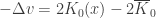
 is the average of
  over
over  . Then it is easy to verify that
  solves the following


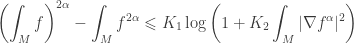
 , the characteristic of
  be an integer and
  -dimensional Riemannian manifold with Ricci curvature bounded below by a positive constant
  . The following inequality holds for
  ,
,  ,
,  ,
, 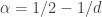 , and
, and  , a smooth function mapping


 satisfies
  in
in 
 . Fix any point
  and consider the function
 as
as  ,
,  is achieved at some
  . We have


 we deduce that
  . In other words,
  .
.


 is a differential of

 . Obviously,
 and that

 , the variation of the Riemann tensor can be calculated as,
 is the difference of two connections, it is a tensor and we can thus calculate its covariant derivative,

