In mathematics, the Poincaré inequality is a result in the theory of Sobolev spaces, named after the French mathematician Henri Poincaré. The inequality allows one to obtain bounds on a function using bounds on its derivatives and the geometry of its domain of definition. Such bounds are of great importance in the modern, direct methods of the calculus of variations. A very closely related result is the Friedrichs’ inequality.
This topic will cover two versions of the Poincaré inequality, one is for  spaces and the other is for
  spaces.
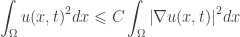
The classical Poincaré inequality for spaces. Assume that  and that
  is a bounded open subset of the
  –dimensional Euclidean space
  with a Lipschitz boundary (i.e., is an open, bounded Lipschitz domain). Then there exists a constant
  , depending only on and
  , such that for every function
  in the Sobolev space ,
 ,
,
where

is the average value of over , with  standing for the Lebesgue measure of the domain .
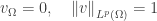
Proof. We argue by contradiction. Were the stated estimate false, there would exist for each integer  a function
  satisfying
 .
.
We renormalize by defining
 .
.
Then

and therefore
 .
.
In particular the functions  are bounded in .
By mean of the Rellich-Kondrachov Theorem, there exists a subsequence  and a function
  such that
 in
in  .
.
Passing to a limit, one easily gets
 .
.
On the other hand, for each  and
and  ,
,
 .
.
Consequently,  with
with  a.e. Thus
  is constant since is connected. Since
  then
then  . This contradicts to
  .
.
The Poincaré inequality for  spaces. Assume that is a bounded open subset of the -dimensional Euclidean space with a Lipschitz boundary (i.e., is an open, bounded Lipschitz domain). Then there exists a constant , depending only on such that for every function in the Sobolev space ,
 .
.
Proof. Assume can be enclosed in a cube
 .
.
Then for any  , we have
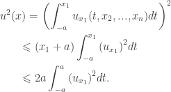 .
.
Thus
 .
.
Integration over  from
from  to
to  gives the result.
The Poincaré inequality for  spaces. Assume that
  and that is a bounded open subset of the -dimensional Euclidean space with a Lipschitz boundary (i.e., is an open, bounded Lipschitz domain). Then there exists a constant , depending only on and , such that for every function in the Sobolev space ,
 ,
,
where  is defined to be
  .
.
Proof. The proof of this version is exactly the same to the proof of case.
Remark. The point  on the boundary of is important. Otherwise, the constant function will not satisfy the Poincaré inequality. In order to avoid this restriction, a weight has been added like the classical Poincaré inequality for case. Sometimes, the Poincaré inequality for spaces is called the Sobolev inequality.


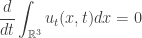


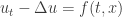
 . Today, we consider another phenomena. Let assume
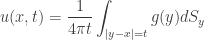
  be an open set with smooth boundary and suppose
  is a solution of

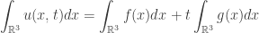
 . Assume that
 .
. .
.
 is constant. For any
  , by the Young inequality, it holds that
 .
. we obtain
 .
. .
. .
. satisfies
 .
. .
.
 ,
, .
. .
. .
.

 .
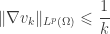
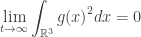
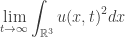
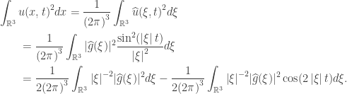
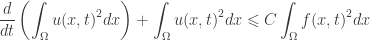
. . We will prove the following estimate
 implies the existence of two positive constants
  and
and  such that
 .
. .
. is less than or equals to the area of
  . Therefore, we obtain
 .
.

 .
. is bounded, continuous, and satisfies
 .
.
 and
and  .
. .
. .
. in the second integral of the above inequality. Then we get immediately
 .
.
 .
.
 of
of  .
. .
. .
. , we can rewrite this one in terms of
  . Actually, we have the following
 .
. and radius
  by
by .
. .
. .
. .
. , then
  as well, where
  . In addition,
  sends a set of small diameter not too close to
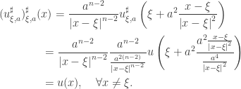

 . Unlike the heat equations in 1D, we cannot illustrate the solution
  . The way to solve this equation numerically is to use, for example, the
  the difference in time, if we have already known the solution
  , then we can solve
  . The Backward Euler Method applied to this model equation gives
 .
. , the solution
  which is actually
  . The time-discretization equation is then given by
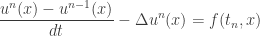 .
. is a
is a  the finite-dimensional subspace of
  with a basis
  such that for each
  , the restriction of
  into
into 
 for every vertices
  at the
  -node are chosen so that
  and
and  for every
  .
.

 .
.
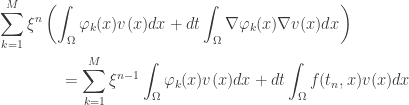 .
. being
being  , we then have
 .
. where
where
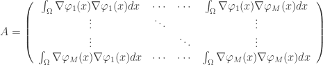
 .
.
 is the function sampled at quadrature point
  on the triangle, and
  is the quadrature weight for that point. The quadrature operation results in a quantity that is normalized by the triangle’s area
  , hence the
  coefficient.
 ,
,  and
and  , any point
  inside that triangle can be written in terms of the barycentric coordinates
  ,
,  and
and  as
as .
.
 is a constant and
  has some special form. The advantage of the method is that it does not require any integrations and is therefore quick to use. The homogeneous equation
 .
. ,
, . If
. If  .
. .
. in a similar form
 .
. .
. .
. .
. ,
, .
. is a polynomial of degree
  is a polynomial of degree
  . If
. If  .
. , so we look for a solution in the same form
  . This leads to
  , and
, and .
. .
. ,
,  ,
,  . So a particular solution is
 .
. .
. , since it would involve a division by zero. More generally, if the equation reads
 , with
  an nth degree polynomial, then we can find a particular solution
 ,
, is some other nth degree polynomial as long as
  . If, on the other hand,
  .
.

 is a given continuous function. The left side of the PDE is a total derivative along the curves in the
  plane defined by the differential equation
 .
.
 on
on  gives the speed of these characteristic curves, which varies in spacetime.


 .
. .
. . We have the following pictures.
 This picture shows the shape of solution in the spacetime.