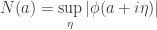
Ngô Quốc Anh

September 29, 2010

The Three Lines Theorem by Hadamard

Filed under: Uncategorized — Tags: — Ngô Quốc Anh @ 11:56

Theorem. Let \phi(\xi) be a bounded analytic function in the strip 0 \leqslant {\rm Re } \, \xi \leqslant 1. Denote

\displaystyle N(a)=\sup_\eta|\phi (a+i\eta)|.

Then

\displaystyle N(a) \leqslant N^{1-a}(0)N^a(1)

Proof. Set c=\log \frac{N(0)}{N(1)}. By the hypothesis, the function \phi(\xi)e^{c\xi} is in absolute value \leqslant N(0) for {\rm Re } \, \xi=0 and {\rm Re } \, \xi=1. So, by the maximum principle applied in the strip 0\leqslant {\rm Re } \, \xi\leqslant 1,

\displaystyle |\phi(a+i\eta)|e^{ca} \leqslant N(0);

from this and the definition of c, the inequality follows.

Source: Functional Analysis by Peter Lax.

September 26, 2010

Subharmonic functions

Filed under: Giải tích 7 (MA4247) — Ngô Quốc Anh @ 1:53

In this entry, we shall discuss a geometric meaning of subharmonic functions. This will help us to easily remember the definition of subharmonic functions.

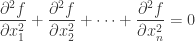
In mathematics, a harmonic function is a twice continuously differentiable function f : U\to \mathbb R (where U is an open subset of \mathbb R^n) which satisfies Laplace’s equation, i.e.

\displaystyle\frac{\partial^2f}{\partial x_1^2} + \frac{\partial^2f}{\partial x_2^2} + \cdots + \frac{\partial^2f}{\partial x_n^2} = 0

everywhere on U. This is usually written as

\textstyle \Delta f = 0.

In 1D, this condition is about to say that f is harmonic if and only if f is linear. Concerning to the case of functions with one-variable, we have the s0-called convexity saying that function f is convex if and only if the function lies below or on the straight line segment connecting two points, for any two points in the interval. Mathematically, a function f is said to be convex if

\textstyle \Delta f \geqslant 0.

In higher dimension, the notion of linearity and convexity become harmonicity and subharmonicity. Precisely, two points mentioned above become a hyper-surface, for e.g. like a curve in 2D and a straight line becomes a graph of harmonic function. In practice, the closed interval connecting those two points will be replaced by a closed ball. Therefore, we have

Definition. A C^2 function that satisfies \Delta f \ge 0 is called subharmonic. More generally, a function is subharmonic if and only if, in the interior of any ball in its domain, its graph lies below that of the harmonic function interpolating its boundary values on the ball.

Let us consider several examples in 2D.

  • \log functions.

It is well-known that in 2D function \log|z|, where z=(x,y), is harmonic. Therefore, every functions lying below the graph of \log|z| turns out to be subharmonic.

  • \sin functions.

Again, one can easily show that e^x \sin y is harmonic.

September 22, 2010

An identity of differentiation involving the Kelvin transform

Filed under: Các Bài Tập Nhỏ, Giải Tích 1 — Tags: — Ngô Quốc Anh @ 15:47

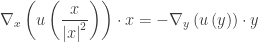
This short note is to prove the following

\displaystyle {\nabla _x}\left( {u\left( {\frac{x}{{{{\left| x \right|}^2}}}} \right)} \right) \cdot x = - {\nabla _y}\left( {u\left( y \right)} \right) \cdot y

where x and y are connected by

\displaystyle y = \frac{x}{{{{\left| x \right|}^2}}} \in {\mathbb{R}^2}.

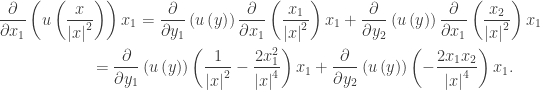
The proof is straightforward as follows.

  • Calculation of \frac{\partial}{\partial x_1}.

We see that

\displaystyle\begin{gathered} \frac{\partial }{{\partial {x_1}}}\left( {u\left( {\frac{x}{{{{\left| x \right|}^2}}}} \right)} \right){x_1} = \frac{\partial }{{\partial {y_1}}}\left( {u\left( y \right)} \right)\frac{\partial }{{\partial {x_1}}}\left( {\frac{{{x_1}}}{{{{\left| x \right|}^2}}}} \right){x_1} + \frac{\partial }{{\partial {y_2}}}\left( {u\left( y \right)} \right)\frac{\partial }{{\partial {x_1}}}\left( {\frac{{{x_2}}}{{{{\left| x \right|}^2}}}} \right){x_1} \hfill \\ \qquad\qquad\qquad= \frac{\partial }{{\partial {y_1}}}\left( {u\left( y \right)} \right)\left( {\frac{1}{{{{\left| x \right|}^2}}} - \frac{{2x_1^2}}{{{{\left| x \right|}^4}}}} \right){x_1} + \frac{\partial }{{\partial {y_2}}}\left( {u\left( y \right)} \right)\left( { - \frac{{2{x_1}{x_2}}}{{{{\left| x \right|}^4}}}} \right){x_1}. \hfill \\ \end{gathered}

  • Calculation of \frac{\partial}{\partial x_2}.

Similarly, we get

\displaystyle\begin{gathered} \frac{\partial }{{\partial {x_2}}}\left( {u\left( {\frac{x}{{{{\left| x \right|}^2}}}} \right)} \right){x_2} = \frac{\partial }{{\partial {y_1}}}\left( {u\left( y \right)} \right)\frac{\partial }{{\partial {x_2}}}\left( {\frac{{{x_1}}}{{{{\left| x \right|}^2}}}} \right){x_2} + \frac{\partial }{{\partial {y_2}}}\left( {u\left( y \right)} \right)\frac{\partial }{{\partial {x_2}}}\left( {\frac{{{x_2}}}{{{{\left| x \right|}^2}}}} \right){x_2} \hfill \\ \qquad\qquad\qquad= \frac{\partial }{{\partial {y_1}}}\left( {u\left( y \right)} \right)\left( { - \frac{{2{x_1}{x_2}}}{{{{\left| x \right|}^4}}}} \right){x_2} + \frac{\partial }{{\partial {y_2}}}\left( {u\left( y \right)} \right)\left( {\frac{1}{{{{\left| x \right|}^2}}} - \frac{{2x_2^2}}{{{{\left| x \right|}^4}}}} \right){x_2}. \hfill \\ \end{gathered}

(more…)

September 18, 2010

Asympotic behavior of integrals, 3

Filed under: PDEs — Tags: — Ngô Quốc Anh @ 11:56

In the previous entry, we showed the following

Theorem. Let u and f be two smooth functions on \mathbb R^2 satisfying

\Delta u(x)=f(x), \quad x \in \mathbb R^2.

Suppose that f is bounded and also f \in L^1(\mathbb R^2) and

|u(x)| \leqslant o(|x|), \quad |x| \to \infty.

Then

\displaystyle\mathop {\lim }\limits_{|x| \to \infty } \frac{{u(x)}}{{\log |x|}} = \frac{1}{{2\pi }}\int_{{\mathbb{R}^2}} {f(y)dy}.

As suggested in an earlier entry, in this topic, we show that the following limit

\displaystyle\mathop {\lim }\limits_{|x| \to \infty } \left[ {u(x) - \alpha \log |x|} \right]

exists where

\displaystyle\alpha = \frac{1}{{2\pi }}\int_{{\mathbb{R}^2}} {f(y)dy}

for some good f.

(more…)

September 14, 2010

Asympotic behavior of integrals, 2

Filed under: Giải Tích 6 (MA5205), PDEs — Tags: — Ngô Quốc Anh @ 15:07

We now prove the following result

Theorem. Let u and f be two smooth functions on \mathbb R^2 satisfying

\Delta u(x)=f(x), \quad x \in \mathbb R^2.

Suppose that f is bounded and also f \in L^1(\mathbb R^2) and

|u(x)| \leqslant o(|x|), \quad |x| \to \infty.

Then

\displaystyle\mathop {\lim }\limits_{|x| \to \infty } \frac{{u(x)}}{{\log |x|}} = \frac{1}{{2\pi }}\int_{{\mathbb{R}^2}} {f(y)dy} .

(more…)

September 10, 2010

MuPAD: Drawing a surface with a line on

Filed under: Uncategorized — Tags: — Ngô Quốc Anh @ 14:21

I took me years to figure out how did we plot such a picture in this entry. Thanks to MuPAD, we can do it quite easily. What I got is the following

Firstly, we need to choose a function which has a mountain-pass shape. Thank to a special solution to the Toda system considered in this entry, we can choose

\displaystyle u(z) = \log \frac{{4\left( {1 + 4{{\left| z \right|}^2} + {{\left| {{z^2} + 2z} \right|}^2}} \right)}}{{{{\left( {1 + {{\left| {z + 1} \right|}^2} + {{\left| {{z^2}} \right|}^2}} \right)}^2}}}, \quad z \in \mathbb R^2.

(more…)

September 7, 2010

Asympotic behavior of integrals

Filed under: Giải Tích 6 (MA5205), PDEs — Tags: — Ngô Quốc Anh @ 10:52

Long time ago, we studied [here] the following fact

Suppose f \in L^1(\mathbb R^n) \cap L_{loc}^\infty (\mathbb R^n) with f \geq 0. Define

\displaystyle Sf\left( x \right) = \int_{\mathbb{R}^n } {\log \frac{{\left| y \right|}}{{\left| {x - y} \right|}}f\left( y \right)dy}.

Show that Sf(x) is finite for all x \in \mathbb R^n and Sf \in L_{loc}^1(\mathbb R^n).

In this entry, from now on we continue to prove several useful results appearing in PDE. We shall prove the following

Theorem. Assume u is a solution to

\displaystyle (-\Delta)^\frac{3}{2} u(x)=-2e^{3u(x)}, \quad x \in \mathbb R^3

with finite energy

\displaystyle \int_{{\mathbb{R}^3}} {{e^{3u(x)}}dx} < \infty.

Then

\displaystyle\mathop {\lim }\limits_{|x| \to \infty } \frac{{u(x)}}{{\log |x|}} = - \frac{1}{{{\pi ^2}}}\int_{{\mathbb{R}^3}} {{e^{3u(y)}}dy} .

(more…)

September 4, 2010

CE: Convergence of improper integrals does not imply the integrands go to zero

Filed under: Counter-examples, Giải Tích 3 — Ngô Quốc Anh @ 12:31

This entry devotes a similar question that raises during a course of series. We all know that for a convergent series of (positive) real number

\displaystyle \sum_{n=1}^\infty a_n

it is necessary to have

\displaystyle\mathop {\lim }\limits_{n \to \infty } {a_n} = 0.

This is the so-called n-th term test. A natural extension is the following question

Question. Suppose f(x) is positive on [0,\infty) and

\displaystyle\int_0^{ + \infty } {f(x)dx}

exists. Must f(x) tend to zero as x \to +\infty?

(more…)

September 1, 2010

The inverse of the Laplace transform by contour integration

Filed under: Giải tích 7 (MA4247) — Ngô Quốc Anh @ 17:23

Usually, we can find the inverse of the Laplace transform \mathcal L[\cdot](s) by looking it up in a table. In this entry, we show an alternative method that inverts Laplace transforms through the powerful method of contour integration.

Consider the piece-wise differentiable function f(x) that vanishes for x < 0. We can express the function e^{-cx}f(x) by the complex Fourier representation of

\displaystyle f(x){e^{ - cx}} = \frac{1}{{2\pi }}\int_{ - \infty }^\infty {{e^{i\omega x}}\left[ {\int_0^\infty {{e^{ - ct}}f(t){e^{ - i\omega t}}dt} } \right]d\omega }

for any value of the real constant c, where the integral

\displaystyle I = \int_0^\infty {{e^{ - ct}}|f(t)|dt}

exists. By multiplying both sides of first equation by e^{cx} and bringing it inside the first integral

\displaystyle f(x) = \frac{1}{{2\pi }}\int_{ - \infty }^\infty {{e^{(c + i\omega )x}}\left[ {\int_0^\infty {f(t){e^{ - (c + i\omega )t}}dt} } \right]d\omega } .

With the substitution z = c+\omega i, where z is a new, complex variable of integration,

\displaystyle f(x) = \frac{1}{{2\pi }}\int_{c - \infty i}^{c + \infty i} {{e^{zx}}\left[ {\int_0^\infty {f(t){e^{ - zt}}dt} } \right]d\omega }.

The quantity inside the square brackets is the Laplace transform \mathcal L[f](z). Therefore, we can express f(t) in terms of its transform by the complex contour integral

(more…)

Blog at WordPress.com.