Ngô Quốc Anh

August 29, 2009

On a polynomials of degree n, having all its zeros in the unit dis


I found a very useful inequality involving a polynomials of degree n, having all its zeros in the unit disk from the following paper, doi:10.1016/j.jmaa.2009.07.049, published in J. Math. Anal. Appl.

Statement. If P(z) is a polynomial of degree n, having all its zeros in the disk |z| \leq 1, then

\left| {zP'(z)} \right| \geq \displaystyle\frac{n} {2}\left| {P(z)} \right|

for |z|=1.

Proof. Since all the zeros of P(z) lie in $latex|z| \leq 1$. Hence if z_1, z_2,...,z_n are the zeros of P(z), then |z_j| \leq 1 for all j =1,2,...,n. Clearly,

\displaystyle\Re \frac{{{e^{i\theta }}P'\left( {{e^{i\theta }}} \right)}}{{P\left( {{e^{i\theta }}} \right)}} = \sum\limits_{j = 1}^n {\Re \frac{{{e^{i\theta }}}}{{{e^{i\theta }} - {z_j}}}} ,

for every point e^{i\theta}, 0 \leq \theta < 2 \pi which is not a zero of P(z). Note that

\displaystyle\sum\limits_{j = 1}^n {\Re \frac{e^{i\theta }}{e^{i\theta } - z_j}}\geq\sum\limits_{j = 1}^n{\frac{1}{2}}=\frac{n}{2}.

This implies

\displaystyle\left| {\frac{{{e^{i\theta }}P'\left( {{e^{i\theta }}} \right)}}{{P\left( {{e^{i\theta }}} \right)}}} \right| \geq \Re \frac{{{e^{i\theta }}P'\left( {{e^{i\theta }}} \right)}}{{P\left( {{e^{i\theta }}} \right)}} \geq \frac{n}{2},

for every point e^{i \pi}, 0 \leq \theta < 2\pi. Hence

\left| {zP'(z)} \right| \geq \displaystyle \frac{n}{2}\left| {P(z)} \right|

for |z|=1 and this completes the proof.

August 18, 2009

An other limit supremum of sin function


In the topic we showed that for any irrational \alpha the limit

\mathop {\lim }\limits_{n \to \infty } \sin \left( {n\alpha \pi } \right)

does not exist. In this topic, we consider the following limit

\mathop {\overline {\lim } }\limits_{n \to \infty } \sin \left( {nx} \right) .

To be precise, we prove that

\mathop {\overline {\lim } }\limits_{n \to \infty } \sin \left( {nx} \right) = 1

for almost every x \in [0,2\pi].

Solution. Let

\displaystyle A = \left\{ {x \in \left( {0,2\pi } \right): \frac{x} {\pi } \notin \mathbb{Q}} \right\}.

Then A is a measurable set of measure 2\pi. Moreover, for any x \in A,

\displaystyle\mathop {\overline {\lim } }\limits_{n \to \infty } \sin \left( {nx} \right) = 1.

Indeed for any x \in A, since

\displaystyle\left\{ {k\frac{x} {\pi } - 2l: l \in \mathbb{Z}} \right\}

is dense subgroup of \mathbb R there are sequences \{k_n\} and \{l_n\} of \mathbb Z such that

\displaystyle \mathop {\lim }\limits_{n \to \infty } \left( {{k_n}\frac{x} {\pi } - {l_n}} \right) = \frac{1} {2}.

Since

\displaystyle \frac{1} {2} \notin \left\{ {k\frac{x} {\pi } - 2l: k,l \in \mathbb{Z}} \right\}

\{k_n\} admits a subsequence \{k'_n\} either increasing to +\infty or decreasing to -\infty. If \mathop {\lim }\limits_{n \to \infty } {{k'}_n} = + \infty then

\mathop {\lim }\limits_{n \to \infty } \sin \left( {{{k'}_n}x} \right) = \mathop {\lim }\limits_{n \to \infty } \sin \left( {...

Otherwise \mathop {\lim }\limits_{n \to \infty } \left( { - 3{{k'}_n}} \right) = + \infty and

\mathop {\lim }\limits_{n \to \infty } \sin \left( { - 3{{k'}_n}x} \right) = \mathop {\lim }\limits_{n \to \infty } \sin \lef...

August 17, 2009

The use of equivalence in measure


In mathematics, and specifically in measure theory, equivalence is a notion of two measures being “the same”. Two measures are equivalent if they have the same null sets.

Definition. Let (X, \Sigma) be a measurable space, and let \mu, \nu : \Sigma \to [0, +\infty] be two measures. Then \mu is said to be equivalent to \nu if

\mu (A) = 0 \iff \nu (A) = 0

for measurable sets A in \Sigma, i.e. the two measures have precisely the same null sets. Equivalence is often denoted \displaystyle{\mu \sim \nu} or \mu \approx \nu.

In terms of absolute continuity of measures, two measures are equivalent if and only if each is absolutely continuous with respect to the other:

\mu \sim \nu \iff \mu \ll \nu \ll \mu.

Equivalence of measures is an equivalence relation on the set of all measures \Sigma \to [0, +\infty].

Examples.

  1. Gaussian measure and Lebesgue measure on the real line are equivalent to one another.
  2. Lebesgue measure and Dirac measure on the real line are inequivalent.

Application. Let \mu be a finite measure on \mathbb R, and define

f\left( x \right) = \int\limits_{ - \infty }^{ + \infty } {\frac{{\ln \left| {x - t} \right|}} {{\sqrt {\left| {x - t} \right...

Show that f(x) is finite a.e. with respect to the Lebesgue measure on \mathbb R.

Proof. Let

g\left( x \right) = \left\{ \begin{gathered}   \frac{{\ln \left| x \right|}} {{\sqrt {\left| x \right|} }},x \ne 0, \hfill \\...

then g \in L^1(\mathbb R, d\nu) where

d\nu \left( x \right) = \frac{{dx}} {{1 + {x^2}}}

and

f\left( x \right) = \int_{ - \infty }^{ + \infty } {g\left( {x - t} \right)d\mu \left( t \right)} ,x \in \mathbb{R}.

Clearly

\int_{ - \infty }^{ + \infty } {\left| {f\left( x \right)} \right|d\mu \left( x \right)}  \leqslant \int_{ - \infty }^{ + \in...

and by Fubini’s Theorem

\int_{ - \infty }^{ + \infty } {\left( {\int_{ - \infty }^{ + \infty } {\left| {g\left( {x - t} \right)} \right|d\mu \left( t...

then

\int_{ - \infty }^{ + \infty } {\left| {f\left( x \right)} \right|d\mu \left( x \right)}  \leqslant \int_{ - \infty }^{ + \in...

Since

\begin{gathered}   \int\limits_{ - \infty }^{ + \infty } {\left( {\int\limits_{ - \infty }^{ + \infty } {\left| {g\left( {x -...

Thus the following function

x \mapsto \int\limits_{ - \infty }^{ + \infty } {\left| {g\left( {x - t} \right)} \right|d\mu \left( t \right)}

finite a.e. with respect to the measure \nu. The conclusion follows from that the measure \nu and the Lebesgue measure are equivalent.

Source: http://en.wikipedia.org/wiki/Equivalence_(measure_theory)

August 16, 2009

On the stability of the Runge-Kutta 4 (RK4)


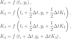
In the literature, the so-called RK4 is given as following: we first define the following coefficients

\displaystyle \begin{gathered}{K_{1}}= f\left({{t_{i}},{y_{i}}}\right),\hfill\\ {K_{2}}= f\left({{t_{i}}+\frac{1}{2}\Delta t,{y_{i}}+\frac{1}{2}\Delta t{K_{1}}}\right),\hfill\\ {K_{3}}= f\left({{t_{i}}+\frac{1}{2}\Delta t,{y_{i}}+\frac{1}{2}\Delta t{K_{2}}}\right),\hfill\\ {K_{4}}= f\left({{t_{i}}+\Delta t,{y_{i}}+\Delta t{K_{3}}}\right),\hfill\\ \end{gathered}

then

\displaystyle {y_{i + 1}} = {y_i} + \frac{{\Delta t}} {6}\left( {{K_1} + 2{K_2} + 2{K_3} + {K_4}} \right).

This is the most important iterative method for the approximation of solutions of ordinary differential equations

\displaystyle y' = f(t, y), \quad y(t_0) = y_0.

This technique was developed around 1900 by the German mathematicians C. Runge and M.W. Kutta. In order to study its stability, we use the model problem

\displaystyle y' = \lambda y, \quad \Re \lambda < 0.

In other words, we replace f(t,y) by \lambda y. Then the stability condition for time step \Delta comes from the following condition

\displaystyle \left| \frac{y_{i+1}}{y_i} \right| \leq 1.

Applying the above discussion to RK4 method, we see that

\displaystyle\begin{gathered}{K_{4}}=\lambda\left({{y_{i}}+\Delta t{K_{3}}}\right),\hfill\\ {K_{3}}=\lambda\left({{y_{i}}+\frac{1}{2}\Delta t{K_{2}}}\right),\hfill\\ {K_{2}}=\lambda\left({{y_{i}}+\frac{1}{2}\Delta t{K_{1}}}\right),\hfill\\ {K_{1}}=\lambda{y_{i}},\hfill\\ \end{gathered}

which implies

\displaystyle\begin{gathered}{K_{4}}=\lambda\left({{y_{i}}+\Delta t\lambda\left({{y_{i}}+\frac{1}{2}\Delta t\lambda\left({{y_{i}}+\frac{1}{2}\Delta t{y_{i}}}\right)}\right)}\right) =\lambda{y_{i}}\left({1+\Delta t\lambda\left({1+\frac{1}{2}\Delta t\lambda\left({1+\frac{1}{2}\Delta t}\right)}\right)}\right),\hfill\\ {K_{3}}=\lambda\left({{y_{i}}+\frac{1}{2}\Delta t\lambda\left({{y_{i}}+\frac{1}{2}\Delta t{y_{i}}}\right)}\right) =\lambda{y_{i}}\left({1+\frac{1}{2}\Delta t\lambda\left({1+\frac{1}{2}\Delta t}\right)}\right),\hfill\\ {K_{2}}=\lambda\left({{y_{i}}+\frac{1}{2}\Delta t\lambda{y_{i}}}\right) =\lambda{y_{i}}\left({1+\frac{1}{2}\Delta t\lambda }\right),\hfill\\ {K_{1}}=\lambda{y_{i}},\hfill\\ \end{gathered}

which yields

\displaystyle\begin{gathered}{K_{4}}=\lambda\left({{y_{i}}+\Delta t\lambda\left({{y_{i}}+\frac{1}{2}\Delta t\lambda\left({{y_{i}}+\frac{1}{2}\Delta t{y_{i}}}\right)}\right)}\right) =\lambda{y_{i}}\left({1+\Delta t\lambda\left({1+\frac{1}{2}\Delta t\lambda\left({1+\frac{1}{2}\Delta t}\right)}\right)}\right),\hfill\\ {K_{3}}=\lambda\left({{y_{i}}+\frac{1}{2}\Delta t\lambda\left({{y_{i}}+\frac{1}{2}\Delta t{y_{i}}}\right)}\right) =\lambda{y_{i}}\left({1+\frac{1}{2}\Delta t\lambda\left({1+\frac{1}{2}\Delta t}\right)}\right),\hfill\\ {K_{2}}=\lambda\left({{y_{i}}+\frac{1}{2}\Delta t\lambda{y_{i}}}\right) =\lambda{y_{i}}\left({1+\frac{1}{2}\Delta t\lambda }\right),\hfill\\ {K_{1}}=\lambda{y_{i}},\hfill\\ \end{gathered}

Thus

\displaystyle\frac{{{y_{i+1}}}}{{{y_{i}}}}= 1+\frac{{\Delta t}}{6}\left[{\lambda+2\lambda\left({1+\frac{1}{2}\Delta t\lambda }\right)+2\lambda\left({1+\frac{1}{2}\Delta t\lambda\left({1+\frac{1}{2}\Delta t}\right)}\right)+\lambda\left[{1+\Delta t\lambda\left({1+\frac{1}{2}\Delta t\lambda\left({1+\frac{1}{2}\Delta t}\right)}\right)}\right]}\right]

which is nothing but

\displaystyle\frac{{{y_{i+1}}}}{{{y_{i}}}}= 1+\Delta t\lambda+\frac{{{{\left({\Delta t\lambda }\right)}^{2}}}}{2}+\frac{{{{\left({\Delta t\lambda }\right)}^{3}}}}{6}+\frac{{{{\left({\Delta t\lambda }\right)}^{4}}}}{{24}}.

Therefore, the stability condition is given as follows

\displaystyle \left| {1 + z + \frac{{{z^2}}} {2} + \frac{{{z^3}}} {6} + \frac{{{z^4}}} {{24}}} \right| \leq 1, \quad \Re z < 0.

The eigenvalues of a common tridiagonal matrix

Filed under: Các Bài Tập Nhỏ, Linh Tinh, Nghiên Cứu Khoa Học — Ngô Quốc Anh @ 3:36

The eigenvalues of then N \times N tridiagonal matrix

\left( {\begin{array}{*{20}{c}}    a & b & {} & {} & {} & {} & {}  \\    c & a & b & {} &...

are

{\lambda _s} = a + 2\sqrt {bc} \cos \frac{{s\pi }} {{N + 1}}

and its conresponding eigenvector is

{v_s}^T = \left( {{{\left( {\frac{c} {b}} \right)}^{\frac{1} {2}}}\sin \frac{{s\pi }} {{N + 1}},{{\left( {\frac{c} {b}} \righ...

Proof. Let \lambda present an eigenvalue of the given matrix (denoted by A) and v the corresponding eigenvector with components v_1,...,v_N. Then

\left( {\begin{array}{*{20}{c}}    a & b & {} & {} & {} & {} & {}  \\    c & a & b & {} &...

If we defined v_0 = v_{N+1}=0, then we have

c{v_{i - 1}} + \left( {a - \lambda } \right){v_i} + b{v_{i + 1}} = 0,i = \overline {1,N} .

The solution of the above equation is of the form

{v_i} = Bm_1^i + Cm_2^i

where B, C are constants and m_1, m_2 are the roots of the equation

c+(a-\lambda)m + bm^2=0.

Since v_0 = v_{N+1}=0, then 0=B+C and 0 = Bm_1^{N + 1} + Cm_2^{N + 1}. Hence,

{\left( {\frac{{{m_1}}} {{{m_2}}}} \right)^{N + 1}} = 1 = {e^{\sqrt { - 1} i2\pi }}

or

\frac{{{m_1}}} {{{m_2}}} = {e^{\frac{{\sqrt { - 1} i2\pi }} {{N + 1}}}}.

We also have

{m_1}{m_2} = \frac{c} {b}, \quad {m_1} + {m_2} = \frac{{\lambda  - a}} {b}.

Finally,

\lambda  = a + b\sqrt {\frac{c} {b}} \left( {{e^{\frac{{\sqrt { - 1} i2\pi }} {{N + 1}}}} + {e^{ - \frac{{\sqrt { - 1} i2\pi ...

The j-component of the eigenvector is

{v_j} = Bm_1^j + Cm_2^j = B\sqrt {{{\left( {\frac{c} {b}} \right)}^j}} \left( {{e^{\frac{{\sqrt { - 1} i2\pi }} {{N + 1}}}} -...

August 15, 2009

Summation by parts (Abel sum formula)


Suppose \{f_k\} and \{g_k\} are two sequences. Then,

\displaystyle\sum_{k=m}^n f_k(g_{k+1}-g_k) = \left[f_{n+1}g_{n+1} - f_m g_m\right] - \sum_{k=m}^n g_{k+1}(f_{k+1}- f_k).

Using the forward difference operator \Delta, it can be stated more succinctly as

\displaystyle\sum_{k=m}^n f_k\Delta g_k = \left[f_{n+1} g_{n+1} - f_m g_m\right] - \sum_{k=m}^n g_{k+1}\Delta f_k,

Note that summation by parts is an analogue to the integration by parts formula,

\displaystyle\int f\,dg = f g - \int g df.

We also have the following identity

\displaystyle\sum_{k=m}^n f_k(g_k-g_{k-1}) = \left[f_{n+1}g_n - f_m g_{m-1}\right] - \sum_{k=m}^n g_k(f_{k+1}- f_k).

Using the backward difference operator \Delta, it can be stated more succinctly as

\displaystyle\sum_{k=m}^n f_k\Delta g_{k-1} = \left[f_{n+1}g_n - f_m g_{m-1}\right] - \sum_{k=m}^n g_k \Delta f_k.

Several questions involving the Vitali set


We denote by V the Vitali set which is defined as follows:

We say that x, y \in  [0, 1) are equivalent, and write x  \sim y, if and only if x - y is a rational number. This equivalence relation partitions [0, 1) into an uncountable family of disjoint equivalence classes. By the axiom of choice there is a set V which contains exactly one element from each equivalence class.

Now let \{ \tau_n\} be a sequence of all rationals in [0, 1) with \tau_0 =0 and define V_n = V + \tau_n (mod 1).

Now we show that the V_n are pairwise disjoint and

\bigcup\limits_n {V_n }  = \left[ {0,1} \right).

Indeed, if x \in V_i \cap V_j, then x = v_i+\tau_i (mod 1) and x = v_j+\tau_j (mod 1), with v_i and v_j belonging to V = V_0. Consequently, v_i - v_j \in \mathbb Q, which means that v_i \sim v_j and therefore i = j. This shows that V_i \cap V_j = 0 if i \ne j. Since each x  \in [0, 1) is in some equivalence class, x differs modulo 1 from an element in V by a rational number, say r, in [0, 1). Thus x \in V_k, which proves that

[0, 1) \subset \bigcup\limits_n {V_n }.

The opposite inclusion is obvious.

Question 1. Show that there exist sets E_1, E_2, ...,E_k,... such that E_k  \searrow E, and |E_k|_e < \infty and

\lim_{k \to \infty} |E_k|_e > |E|_e

with strict inequality.

Solution. We put E_n  = \bigcup\limits_{k \geq n} {V_k }. Clearly, \{E_n\} is a decreasing sequence. Since the V_k are pairwise disjoint, we see that E: = \bigcap\limits_n {E_n }  = \emptyset and E_n  \searrow E. Moreover,

\left| {E_n } \right|_e  \geq  \left| {V_n } \right|_e  = \left| V \right|_e  > 0

(the last inequality comes from the fact that V is not measurable). It is now enough to show that

\mathop {\lim }\limits_{n \to \infty } \left| {E_n } \right|_e  \geq  \left| V \right|_e  > 0 = \left| E \right|_e

and the proof is complete.

Question 2. Show that there exist disjoint E_1, E_2, ...,E_k,... such that

\left| { \bigcup_k E_k } \right|_e  < \sum_k {\left| {E_k } \right|_e }

with strict inequality.

Solution. We put E_n = V_n then E_n are pairwise disjoint and obviously

\left| {\bigcup_n {E_n } } \right|_e  = \left| {\left[ {0,1} \right)} \right|_e  = 1.

Moreover, all the E_n are of the same outer measure. Thus \sum_n {\left| {E_n } \right|_e }  =  + \infty which completes the proof.

Question 3. Show that each of the sets

{E_n} = \bigcup\limits_{k = 0}^n {{V_k}}

is non-measurable.

Question 4. Show that if E is a measurable subset of the Vitali set V, then |E|=0.

Question 5. Show that there exist sets A and B such that

{\left| {A \cup B} \right|_i} = {\left| A \right|_i} + {\left| B \right|_i}

but

{\left| {A \cup B} \right|_e} < {\left| A \right|_e} + {\left| B \right|_e}.

Question 6. Show that any set of positive outer measure contains a non-measurable subset.

August 14, 2009

How to find a conformal mapping between the quadrants and the semidisc


In the previous topic I show you by the following map

\displaystyle f : z \mapsto \frac{z+1}{z-1}

maps \{z : \Re z < 0\} onto \{w : |w|<1\}, and is conformal. Therefore the map

\displaystyle g : z \mapsto \frac{z+1}{1-z}

maps \{z : \Re z > 0\} onto \{w : |w|<1\}, and is conformal. What I am going to do is to prove that

\displaystyle \Re z > 0\quad \Leftrightarrow \quad \Re \left( {\frac{{z + 1}} {{1-z}}} \right) > 0.

To this purpose, we assume z=x+iy, i.e., \Re z = y. Now by a simple calculation

\displaystyle\frac{{z+1}}{{1-z}}=\frac{{\left({x+1}\right)+iy}}{{\left({1-x}\right)-iy}}=\frac{{\left[{\left({x+1}\right)+iy}\right]\left[{\left({1-x}\right)+iy}\right]}}{{{{\left({1-x}\right)}^{2}}+{y^{2}}}}

which yields

\displaystyle \Re \left( {\frac{{z + 1}} {{1 - z}}} \right) = \frac{{2y}} {{{{\left( {1 - x} \right)}^2} + {y^2}}}.

Having this fact we can easily see that under the map g the first and fourth quadrants maps to upper and lower semidisks, respectively.

An easy way to construct a conformal mapping between upper half plane and the open unit disk


Thelocus |z + 1|= | z -1| is the perpendicular bisector of the line segment joining -1 to 1, that is, the imaginary axis. The set |z + 1|< | z -1| is then the set of points z closer to -1 than to 1, that is, the left half-plane \Re z <0. Hence, \Re z <0 if and only if

\displaystyle\frac{|z+1|}{|z-1|}<1.

The map

\displaystyle f : z \mapsto \frac{z+1}{z-1}

maps \{z : \Re z < 0\} onto \{w : |w|<1\}, and is conformal as f' \ne 0. The inverse map is easily seen to be

\displaystyle w \mapsto z=\frac{w+1}{w-1}.

The locus |z + i|= | z - i| is the perpendicular bisector of the line segment joining -i to i, that is, the real axis. The set |z + i|< | z -i| is then the set of points z closer to -i than to i, that is, the lower half-plane \Im z <0. Hence, \Im z <0 if and only if

\displaystyle \frac{|z+i|}{|z-i|}<1.

The map

\displaystyle g : z \mapsto \frac{z+i}{z-i}

maps \{z : \Im z < 0\} onto \{w : |w|<1\}, and is conformal as g' \ne 0. The inverse map is easily seen to be

\displaystyle w \mapsto z=\frac{w+1}{w-1}i.

August 13, 2009

Two examples of analytic function on a punctured unit disk which has a removable singularity at the origin

Filed under: Các Bài Tập Nhỏ, Giải tích 7 (MA4247), Linh Tinh — Ngô Quốc Anh @ 15:54

The following question was proposed in NUS under the QE in AY 2007-2008:

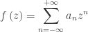
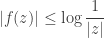
Consider the punctured disk D=\{ z \in \mathbb C | 0 <|z| <1\}. Suppose f : D \to \mathbb C is an analytic function such that

\displaystyle |f''(z)| \leq \frac{2}{|z|^2}

for all z \in D. Is it true that f has a removable singular point at z=0?

Proof. Denote the Laurent expansion of f by

\displaystyle f\left( z \right) = \sum\limits_{n = - \infty }^{ + \infty } {{a_n}{z^n}}

where

\displaystyle {a_n} = \frac{1} {{2\pi i}}\int\limits_{\left| z \right| = r < 1} {\frac{{f\left( z \right)dz}} {{{z^{n + 1}}}}}.

Then from

\displaystyle f''\left( z\right) =\sum\limits_{n =-\infty }^{+\infty }{\underbrace{\left({n+2}\right)\left({n+1}\right){a_{n+2}}}_{{b_{n}}}{z^{n}}}

we get

\displaystyle {b_n} = \frac{1} {{2\pi i}}\int\limits_{\left| z \right| = r < 1} {\frac{{f''\left( z \right)dz}} {{{z^{n + 1}}}}}.

Thus,

\displaystyle\left|{{b_{n}}}\right|\leqslant\frac{1}{{2\pi }}\int\limits_{\left| z\right| = r < 1}{\left|{\frac{{f''\left( z\right)}}{{{z^{n+1}}}}}\right|}dz\leqslant\frac{1}{\pi }\int\limits_{\left| z\right| = r < 1}{\left|{\frac{1}{{{z^{n+3}}}}}\right|}dz\leqslant\frac{1}{{\pi{r^{n+3}}}}2\pi r =\frac{2}{{{r^{n+2}}}}.

When n \leq -3, let r \to 0 we see that z=0 is a removable singularity of f since b_n=0 (n \leq -3) implies a_n=0 (n \leq -1).

Remark. The second derivative can be replaced by an \mathbb Z\ni m \geq 1and therefore \frac{2}{|z|^2} should be \frac{2}{|z|^m}. This is a question of UCLA QE in Winter 2007.

We also have a similar question proposed in a QE of Indiana University. It says that if f : D \to \mathbb C is an analytic function such that

\displaystyle |f(z)|\leq\log\frac{1}{|z|}

for all z \in D. Then f \equiv 0.

Proof
. As above, one has

\displaystyle \left|{{b_{n}}}\right| =\left|{\frac{1}{{2\pi i}}\int\limits_{\left| z\right| = r < 1}{\frac{{f\left( z\right)dz}}{{{z^{n+1}}}}}}\right|\leqslant\frac{1}{{{r^{n}}}}\log\frac{1}{r}.

When n<0, letting r \to 0 we have a_n= 0 for all n \leq -1 which implies z=0 is a removable singularity of f. In other words, f can be extended to an analytic function of the unit disk. Since \log \frac{1}{|z|} =0 when |z|=1, by the Maximum Modules Principle we obtain f \equiv 0.

Older Posts »

Blog at WordPress.com.