A root-finding algorithm is a numerical method, or algorithm, for finding a value  such that
  , for a given function
  . Such an is called a root of the function .
Suppose is a continuous function defined on the interval ![[a, b]](https://s0.wp.com/latex.php?latex=%5Ba%2C+b%5D&bg=ffffff&fg=333333&s=0&c=20201002) , with
, with  and
and  of opposite sign. By the Intermediate Value Theorem, there exists a number
  in
in  with
with  . Although the procedure will work when there is more than one root in the interval
  , we assume for simplicity that the root in this interval is unique. The method calls for a repeated halving of subintervals of and, at each step, locating the half containing .
 To begin, set
  and
and  , and let
  be the midpoint of
 ![[a,b]](https://s0.wp.com/latex.php?latex=%5Ba%2Cb%5D&bg=ffffff&fg=333333&s=0&c=20201002) ; that is,
; that is,
 .
.
If  , then
  , and we are done. If
  , then
  has the same sign as either
  or
or  . When and have the same sign,
  , and we set
  and
and  . When and have opposite signs,
  , and we set
  and
and  . We then reapply the process to the interval
 ![[a_2, b_2]](https://s0.wp.com/latex.php?latex=%5Ba_2%2C+b_2%5D&bg=ffffff&fg=333333&s=0&c=20201002) .
.
A number p is a fixed point for a given function g if  . In this section we consider the problem of finding solutions to fixed-point problems and the connection between the fixed-point problems and the root-finding problems we wish to solve. Root-finding problems and fixed-point problems are equivalent classes in the following sense:
Given a root-finding problem , we can define functions  with a fixed point at in a number of ways, for example, as
  or as
or as  . Conversely, if the function has a fixed point at , then the function defined by
  has a zero at .

Although the problems we wish to solve are in the root-finding form, the fixed-point form is easier to analyze, and certain fixed-point choices lead to very powerful root-finding techniques.

Newton’s (or the Newton-Raphson) method is one of the most powerful and well-known numerical methods for solving aroot-finding problem. With an initial approximation  , the Newton’s method generates the sequence
  by
by
 .
.

To circumvent the problem of the derivative evaluation in Newton’s method, we introduce a slight variation. By definition,
 .
.
Letting  , we have
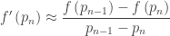
which yields
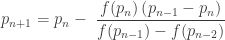 .
.

- The method of False Position
The method of False Position (also called Regula Falsi) generates approximations in the same manner as the Secant method, but it includes a test to ensure that the root is bracketed between successive iterations. Although it is not a method we generally recommend, it illustrates how bracketing can be incorporated.
First choose initial approximations and with  . The approximation
  is chosen in the same manner as in the Secant method, as the -intercept of the line joining
  and
and  . To decide which secant line to use to compute
  , we check
  . If this value is negative, then and bracket a root, and we choose as the -intercept of the line joining and
  . If not, we choose as the -intercept of the line joining and , and then interchange the indices on and .

In a similar manner, once is found, the sign of  determines whether we use and or and to compute
  . In the latter case a relabeling of and is performed.
Source: Richard L. Burden and J. Douglas Faires, Numerical Analysis, 8th edition, Thomson/Brooks/Cole, 2005.


 by a polynomial of order at most
  in terms of derivatives of
  . Both the error of the approximation and the derivatives of
  norms on a bounded domain in
  .
. , there exists a constant
  such that
 where
where  and
and  denote the norm and semi-norm of the
  .
. boundary.
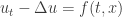 . Unlike the heat equations in 1D, we cannot illustrate the solution
  . The point is
  . The way to solve this equation numerically is to use, for example, the
  the difference in time, if we have already known the solution
  , then we can solve
  . The Backward Euler Method applied to this model equation gives
 .
. we mean we are working on the
  , the solution
  which is actually
  . The time-discretization equation is then given by
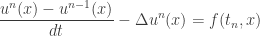 .
. is a
is a  small special triangles. Vertices of triangles, usually called nodes, are those points we want to approximate
  the finite-dimensional subspace of
  with a basis
  such that for each
  , the restriction of
  into
into 
 for every vertices
  at the
  -node are chosen so that
  and
and  for every
  .
.

 .
.
 .
. being
being  , we then have
 .
. where
where
 .
.
 is the function sampled at quadrature point
  on the triangle, and
  is the quadrature weight for that point. The quadrature operation results in a quantity that is normalized by the triangle’s area
  , hence the
  coefficient.
 ,
,  and
and  , any point
  inside that triangle can be written in terms of the barycentric coordinates
  ,
,  and
and  as
as .
. where
where  with boundary conditions
  .
.![[0,1]](https://s0.wp.com/latex.php?latex=%5B0%2C1%5D&bg=ffffff&fg=333333&s=0&c=20201002) into
into  where
where  . We then approximate
  by using the following
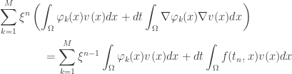
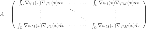
 . Therefore, we have the following system of linear equations
 where
where ![\displaystyle\int_0^1 {\nabla u\nabla vdx} = \int_0^1 {f(x)vdx} ,\quad\forall v \in H_0^1([0,1])](https://s0.wp.com/latex.php?latex=%5Cdisplaystyle%5Cint_0%5E1+%7B%5Cnabla+u%5Cnabla+vdx%7D+%3D+%5Cint_0%5E1+%7Bf%28x%29vdx%7D+%2C%5Cquad%5Cforall+v+%5Cin+H_0%5E1%28%5B0%2C1%5D%29&bg=ffffff&fg=333333&s=0&c=20201002) .
.![f \in L^2([0,1])](https://s0.wp.com/latex.php?latex=f+%5Cin+L%5E2%28%5B0%2C1%5D%29&bg=ffffff&fg=333333&s=0&c=20201002) , the existence of weak solution is well-understood via the Lax-Milgram lemma.
, the existence of weak solution is well-understood via the Lax-Milgram lemma.![[x_{i-1},x_i]](https://s0.wp.com/latex.php?latex=%5Bx_%7Bi-1%7D%2Cx_i%5D&bg=ffffff&fg=333333&s=0&c=20201002) where
where  . We also suppose that
  . Clearly the space
  constructed as follows
![\phi_i \in H_0^1([0,1])](https://s0.wp.com/latex.php?latex=%5Cphi_i+%5Cin+H_0%5E1%28%5B0%2C1%5D%29&bg=ffffff&fg=333333&s=0&c=20201002) .
.
 denoted by
  for every
  . Precisely, let
 .
. by
by  and
and 
 .
. as the following
 .
.
 .
. .
. .
. by
by  . Then the stability condition for time step \Delta comes from the following condition
 .
.

![\displaystyle\frac{{{y_{i+1}}}}{{{y_{i}}}}= 1+\frac{{\Delta t}}{6}\left[{\lambda+2\lambda\left({1+\frac{1}{2}\Delta t\lambda }\right)+2\lambda\left({1+\frac{1}{2}\Delta t\lambda\left({1+\frac{1}{2}\Delta t}\right)}\right)+\lambda\left[{1+\Delta t\lambda\left({1+\frac{1}{2}\Delta t\lambda\left({1+\frac{1}{2}\Delta t}\right)}\right)}\right]}\right]](https://s0.wp.com/latex.php?latex=%5Cdisplaystyle%5Cfrac%7B%7B%7By_%7Bi%2B1%7D%7D%7D%7D%7B%7B%7By_%7Bi%7D%7D%7D%7D%3D+1%2B%5Cfrac%7B%7B%5CDelta+t%7D%7D%7B6%7D%5Cleft%5B%7B%5Clambda%2B2%5Clambda%5Cleft%28%7B1%2B%5Cfrac%7B1%7D%7B2%7D%5CDelta+t%5Clambda+%7D%5Cright%29%2B2%5Clambda%5Cleft%28%7B1%2B%5Cfrac%7B1%7D%7B2%7D%5CDelta+t%5Clambda%5Cleft%28%7B1%2B%5Cfrac%7B1%7D%7B2%7D%5CDelta+t%7D%5Cright%29%7D%5Cright%29%2B%5Clambda%5Cleft%5B%7B1%2B%5CDelta+t%5Clambda%5Cleft%28%7B1%2B%5Cfrac%7B1%7D%7B2%7D%5CDelta+t%5Clambda%5Cleft%28%7B1%2B%5Cfrac%7B1%7D%7B2%7D%5CDelta+t%7D%5Cright%29%7D%5Cright%29%7D%5Cright%5D%7D%5Cright%5D&bg=ffffff&fg=333333&s=0&c=20201002)
 .
. .
. and
and  are two sequences. Then,
![\displaystyle\sum_{k=m}^n f_k(g_{k+1}-g_k) = \left[f_{n+1}g_{n+1} - f_m g_m\right] - \sum_{k=m}^n g_{k+1}(f_{k+1}- f_k)](https://s0.wp.com/latex.php?latex=%5Cdisplaystyle%5Csum_%7Bk%3Dm%7D%5En+f_k%28g_%7Bk%2B1%7D-g_k%29+%3D+%5Cleft%5Bf_%7Bn%2B1%7Dg_%7Bn%2B1%7D+-+f_m+g_m%5Cright%5D+-+%5Csum_%7Bk%3Dm%7D%5En+g_%7Bk%2B1%7D%28f_%7Bk%2B1%7D-+f_k%29&bg=ffffff&fg=333333&s=0&c=20201002) .
. , it can be stated more succinctly as
![\displaystyle\sum_{k=m}^n f_k\Delta g_k = \left[f_{n+1} g_{n+1} - f_m g_m\right] - \sum_{k=m}^n g_{k+1}\Delta f_k](https://s0.wp.com/latex.php?latex=%5Cdisplaystyle%5Csum_%7Bk%3Dm%7D%5En+f_k%5CDelta+g_k+%3D+%5Cleft%5Bf_%7Bn%2B1%7D+g_%7Bn%2B1%7D+-+f_m+g_m%5Cright%5D+-+%5Csum_%7Bk%3Dm%7D%5En+g_%7Bk%2B1%7D%5CDelta+f_k&bg=ffffff&fg=333333&s=0&c=20201002) ,
, .
.![\displaystyle\sum_{k=m}^n f_k(g_k-g_{k-1}) = \left[f_{n+1}g_n - f_m g_{m-1}\right] - \sum_{k=m}^n g_k(f_{k+1}- f_k)](https://s0.wp.com/latex.php?latex=%5Cdisplaystyle%5Csum_%7Bk%3Dm%7D%5En+f_k%28g_k-g_%7Bk-1%7D%29+%3D+%5Cleft%5Bf_%7Bn%2B1%7Dg_n+-+f_m+g_%7Bm-1%7D%5Cright%5D+-+%5Csum_%7Bk%3Dm%7D%5En+g_k%28f_%7Bk%2B1%7D-+f_k%29&bg=ffffff&fg=333333&s=0&c=20201002) .
.![\displaystyle\sum_{k=m}^n f_k\Delta g_{k-1} = \left[f_{n+1}g_n - f_m g_{m-1}\right] - \sum_{k=m}^n g_k \Delta f_k](https://s0.wp.com/latex.php?latex=%5Cdisplaystyle%5Csum_%7Bk%3Dm%7D%5En+f_k%5CDelta+g_%7Bk-1%7D+%3D+%5Cleft%5Bf_%7Bn%2B1%7Dg_n+-+f_m+g_%7Bm-1%7D%5Cright%5D+-+%5Csum_%7Bk%3Dm%7D%5En+g_k+%5CDelta+f_k&bg=ffffff&fg=333333&s=0&c=20201002) .
.
 denote the solution of the initial value problem
 as the difference between
  and the specified boundary value
  .
. 
 has a root, and that root is just the value of
  which yields a solution
  of the boundary value problem. The usual methods for finding roots may be employed here, such as the bisection method or Newton’s method.
 has the form

 is the solution to the initial value problem
 is the solution to the initial value problem
 then
then  for all
  . Thus
  for all
  for all
  ,
, 
 . This is self-satisfied.
 ,
, 
 .
.
 .
.
 , and
, and  plotted in the first figure. Inspecting the plot of
  and
and  . Some trajectories of
  are shown in the second figure.
 and
and  (approximately).

 equal to
  ,
,  ,
,  (red, green, blue, cyan, and magenta, respectively). The point
  is marked with a red diamond.