I want to write a short survey about the Yamabe problem. Long time ago, I introduced the problem in this blog [here] but it turns out that the note was not rich enough to perform the importance of the problem.
Hidehiko Yamabe, in his famous paper entitled On a deformation of Riemannian structures on compact manifolds, Osaka Math. J. 12 (1960), pp. 21-37, wanted to solve the Poincaré conjecture
Conjecture. Every simply connected, closed 3-manifold is homeomorphic to the 3-sphere
For this he thought, as a first step, to exhibit a metric with constant scalar curvature. We refer the reader to this note for details. He considered conformal metrics (the simplest change of metric is a conformal one), and gave a proof of the following statement:
Theorem (Yamabe). On a compact Riemannian manifold
of dimension
, there exists a metric
conformal to
, such that the corresponding scalar curvature
is constant.
As can be seen, the Yamabe problem is a special case of the prescribing scalar curvature problem that can be completely solved. For the prescribing scalar curvature, we also solve it completely when the invariant is non-positive.
1. Conformal metrics.
Definition (conformal). Two pseudo-Riemannian metrics
on a manifold
are said to be
- (pointwise) conformal if there exists a
function
on
;
- conformally equivalent if there exists a diffeomorphism
of
and
Note that, if 

2. Scalar curvature under conformal changes of Riemannian metrics.
We have already shown in this entry that under the conformal change 
![\displaystyle{\rm Scal}_{\widetilde g} = {e^{ - 2f}}\left[ {{\rm Scal}_g - 2(n - 1)\Delta_g f- (n - 2)(n - 1)|{\rm grad} f{|_g^2}} \right].](https://s0.wp.com/latex.php?latex=%5Cdisplaystyle%7B%5Crm+Scal%7D_%7B%5Cwidetilde+g%7D+%3D+%7Be%5E%7B+-+2f%7D%7D%5Cleft%5B+%7B%7B%5Crm+Scal%7D_g+-+2%28n+-+1%29%5CDelta_g+f-+%28n+-+2%29%28n+-+1%29%7C%7B%5Crm+grad%7D+f%7B%7C_g%5E2%7D%7D+%5Cright%5D.&bg=ffffff&fg=333333&s=0&c=20201002)
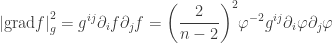
If we consider the conformal deformation in the form 


we then have

In other words,

Thus
and (see this note for a similar calculation for Laplacian)
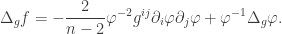
Therefore,

Hence,
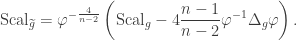
3. The Yamabe approach.
From the previous section, the scalar curvature satisfies the equation

So, Yamabe problem is equivalent to solving the above equation with 

4. The mistake and…
The Yamabe problem was born, since there is a gap in Yamabe’s proof.
See also: Conformal invariant operators: Laplacian operators, 2
- The Yamabe problem: A Story
- The Yamabe problem: The work by Hidehiko Yamabe
- The Yamabe problem: The work by Neil Sidney Trudinger
- The Yamabe problem: The work by Thierry Aubin
- The Yamabe problem: The work by Richard Melvin Schoen

[…] also recommend this short overview of the Yamabe […]
Pingback by Heuristics for the Yamabe Problem – Math Solution — March 13, 2022 @ 7:32