In this entry, we shall discuss a geometric meaning of subharmonic functions. This will help us to easily remember the definition of subharmonic functions.
In mathematics, a harmonic function is a twice continuously differentiable function 


everywhere on

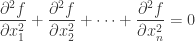
In 1D, this condition is about to say that 

In higher dimension, the notion of linearity and convexity become harmonicity and subharmonicity. Precisely, two points mentioned above become a hyper-surface, for e.g. like a curve in 2D and a straight line becomes a graph of harmonic function. In practice, the closed interval connecting those two points will be replaced by a closed ball. Therefore, we have
Definition. A
function that satisfies
is called subharmonic. More generally, a function is subharmonic if and only if, in the interior of any ball in its domain, its graph lies below that of the harmonic function interpolating its boundary values on the ball.
Let us consider several examples in 2D.
functions.
It is well-known that in 2D function 

functions.
Again, one can easily show that 
](https://s0.wp.com/latex.php?latex=%5Cmathcal+L%5B%5Ccdot%5D%28s%29&bg=ffffff&fg=333333&s=0&c=20201002) by looking it up in a table. In this entry, we show an alternative method that inverts Laplace transforms through the powerful method of contour integration.
by looking it up in a table. In this entry, we show an alternative method that inverts Laplace transforms through the powerful method of contour integration. that vanishes for
  . We can express the function
  by the complex Fourier representation of
![\displaystyle f(x){e^{ - cx}} = \frac{1}{{2\pi }}\int_{ - \infty }^\infty {{e^{i\omega x}}\left[ {\int_0^\infty {{e^{ - ct}}f(t){e^{ - i\omega t}}dt} } \right]d\omega }](https://s0.wp.com/latex.php?latex=%5Cdisplaystyle+f%28x%29%7Be%5E%7B+-+cx%7D%7D+%3D+%5Cfrac%7B1%7D%7B%7B2%5Cpi+%7D%7D%5Cint_%7B+-+%5Cinfty+%7D%5E%5Cinfty+%7B%7Be%5E%7Bi%5Comega+x%7D%7D%5Cleft%5B+%7B%5Cint_0%5E%5Cinfty+%7B%7Be%5E%7B+-+ct%7D%7Df%28t%29%7Be%5E%7B+-+i%5Comega+t%7D%7Ddt%7D+%7D+%5Cright%5Dd%5Comega+%7D+&bg=ffffff&fg=333333&s=0&c=20201002)
 , where the integral
 and bringing it inside the first integral
![\displaystyle f(x) = \frac{1}{{2\pi }}\int_{ - \infty }^\infty {{e^{(c + i\omega )x}}\left[ {\int_0^\infty {f(t){e^{ - (c + i\omega )t}}dt} } \right]d\omega }](https://s0.wp.com/latex.php?latex=%5Cdisplaystyle+f%28x%29+%3D+%5Cfrac%7B1%7D%7B%7B2%5Cpi+%7D%7D%5Cint_%7B+-+%5Cinfty+%7D%5E%5Cinfty+%7B%7Be%5E%7B%28c+%2B+i%5Comega+%29x%7D%7D%5Cleft%5B+%7B%5Cint_0%5E%5Cinfty+%7Bf%28t%29%7Be%5E%7B+-+%28c+%2B+i%5Comega+%29t%7D%7Ddt%7D+%7D+%5Cright%5Dd%5Comega+%7D+&bg=ffffff&fg=333333&s=0&c=20201002) .
. , where
  is a new, complex variable of integration,
![\displaystyle f(x) = \frac{1}{{2\pi }}\int_{c - \infty i}^{c + \infty i} {{e^{zx}}\left[ {\int_0^\infty {f(t){e^{ - zt}}dt} } \right]d\omega }](https://s0.wp.com/latex.php?latex=%5Cdisplaystyle+f%28x%29+%3D+%5Cfrac%7B1%7D%7B%7B2%5Cpi+%7D%7D%5Cint_%7Bc+-+%5Cinfty+i%7D%5E%7Bc+%2B+%5Cinfty+i%7D+%7B%7Be%5E%7Bzx%7D%7D%5Cleft%5B+%7B%5Cint_0%5E%5Cinfty+%7Bf%28t%29%7Be%5E%7B+-+zt%7D%7Ddt%7D+%7D+%5Cright%5Dd%5Comega+%7D&bg=ffffff&fg=333333&s=0&c=20201002) .
.](https://s0.wp.com/latex.php?latex=%5Cmathcal+L%5Bf%5D%28z%29&bg=ffffff&fg=333333&s=0&c=20201002) . Therefore, we can express
. Therefore, we can express  in terms of its transform by the complex contour integral
 be a simply connected domain in
  . Then all real solutions of
 a constant, are of the form
 , it holds
 denotes the standard metric on
  with constant curvature
  and
and
 .
. .
. , the Fourier transform of function
 ![\mathcal F[f]](https://s0.wp.com/latex.php?latex=%5Cmathcal+F%5Bf%5D&bg=ffffff&fg=333333&s=0&c=20201002) , is defined to be
, is defined to be = \int_{ - \infty }^\infty {f(x){e^{ - 2\pi ixy}}dx}](https://s0.wp.com/latex.php?latex=%5Cdisplaystyle+%5Cmathcal+F%5Bf%5D%28y%29+%3D+%5Cint_%7B+-+%5Cinfty+%7D%5E%5Cinfty+%7Bf%28x%29%7Be%5E%7B+-+2%5Cpi+ixy%7D%7Ddx%7D&bg=ffffff&fg=333333&s=0&c=20201002) .
.![\displaystyle\begin{gathered} \mathcal{F}\left[ {\mathcal{F}[f]} \right](z) = \int_{ - \infty }^\infty {\mathcal{F}[f](y){e^{ - 2\pi iyz}}dy} \hfill \\ \qquad\qquad= \int_{ - \infty }^\infty {\mathcal{F}[f](y){e^{2\pi iy( - z)}}dy} \hfill \\ \qquad\qquad= {\mathcal{F}^{ - 1}}\left[ {\mathcal{F}[f]} \right]( - z) \hfill \\ \qquad\qquad= f( - z) \hfill \\ \end{gathered}](https://s0.wp.com/latex.php?latex=%5Cdisplaystyle%5Cbegin%7Bgathered%7D+%5Cmathcal%7BF%7D%5Cleft%5B+%7B%5Cmathcal%7BF%7D%5Bf%5D%7D+%5Cright%5D%28z%29+%3D+%5Cint_%7B+-+%5Cinfty+%7D%5E%5Cinfty+%7B%5Cmathcal%7BF%7D%5Bf%5D%28y%29%7Be%5E%7B+-+2%5Cpi+iyz%7D%7Ddy%7D+%5Chfill+%5C%5C+%5Cqquad%5Cqquad%3D+%5Cint_%7B+-+%5Cinfty+%7D%5E%5Cinfty+%7B%5Cmathcal%7BF%7D%5Bf%5D%28y%29%7Be%5E%7B2%5Cpi+iy%28+-+z%29%7D%7Ddy%7D+%5Chfill+%5C%5C+%5Cqquad%5Cqquad%3D+%7B%5Cmathcal%7BF%7D%5E%7B+-+1%7D%7D%5Cleft%5B+%7B%5Cmathcal%7BF%7D%5Bf%5D%7D+%5Cright%5D%28+-+z%29+%5Chfill+%5C%5C+%5Cqquad%5Cqquad%3D+f%28+-+z%29+%5Chfill+%5C%5C+%5Cend%7Bgathered%7D&bg=ffffff&fg=333333&s=0&c=20201002)
 denotes the inverse Fourier transform.
 with respect to a point
  is defined by
 .
. be open and bounded. Let
  and
and  . Notation
  denotes the Jacobian of
  . It is well-known that the Brouwer Degree Theory, usually denoted by
  , is constructed for continuous function,
  -class, via the following steps
 -class: We assume
  then
then
 -class: In case we want to remove the condition
 is any regular value of
  in the sense that
 .
.
 is sufficiently closed to
  .
. be the unit ball and
  . Assume
 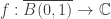 is a
is a  function and
  . Then
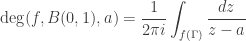 .
. such that
  for all
  is constant.
 for all
  with some positive numbers
  , then
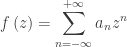
 .
. with
with  are zero, i.e.
 .
. , one has
 .
. we obtain that
  which implies that

 be the open unit disk in the complex plane
  be a holomorphic function with
  . The Schwarz lemma states that under these circumstances
  for all
  , and
, and  . Moreover, if the equality
  holds for any
  , or
, or  then
then  with
with  .
. .
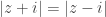
. . The function
  is holomorphic in
  (excluding
  ) since
  be a closed disc within
  . By the maximum modulus principle,
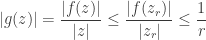
 on the boundary of
  we get
  . Moreover, if there exists a $z_0$ in
  . Then, applying the maximum modulus principle to
  , we obtain that
  , where
  is constant and
  . This is also the case if
  be holomorphic. Then, for all
  ,
,
 .
. , having all its zeros in the unit disk from the following paper, doi:
 is a polynomial of degree
  , then
 .
. are the zeros of
  for all
  . Clearly,
 ,
,  which is not a zero of
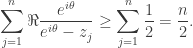
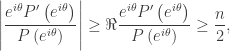
 ,
,  . Hence

 onto
onto  , and is conformal. Therefore the map
 onto
onto  .
. , i.e.,
  . Now by a simple calculation
![\displaystyle\frac{{z+1}}{{1-z}}=\frac{{\left({x+1}\right)+iy}}{{\left({1-x}\right)-iy}}=\frac{{\left[{\left({x+1}\right)+iy}\right]\left[{\left({1-x}\right)+iy}\right]}}{{{{\left({1-x}\right)}^{2}}+{y^{2}}}}](https://s0.wp.com/latex.php?latex=%5Cdisplaystyle%5Cfrac%7B%7Bz%2B1%7D%7D%7B%7B1-z%7D%7D%3D%5Cfrac%7B%7B%5Cleft%28%7Bx%2B1%7D%5Cright%29%2Biy%7D%7D%7B%7B%5Cleft%28%7B1-x%7D%5Cright%29-iy%7D%7D%3D%5Cfrac%7B%7B%5Cleft%5B%7B%5Cleft%28%7Bx%2B1%7D%5Cright%29%2Biy%7D%5Cright%5D%5Cleft%5B%7B%5Cleft%28%7B1-x%7D%5Cright%29%2Biy%7D%5Cright%5D%7D%7D%7B%7B%7B%7B%5Cleft%28%7B1-x%7D%5Cright%29%7D%5E%7B2%7D%7D%2B%7By%5E%7B2%7D%7D%7D%7D&bg=ffffff&fg=333333&s=0&c=20201002)
 .
.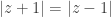 is the perpendicular bisector of the line segment joining
  to
to  is then the set of points
  . Hence,
  .
. . The inverse map is easily seen to be
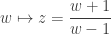 .
. is the perpendicular bisector of the line segment joining
  to
to  , that is, the real axis. The set
  is then the set of points
  . Hence,
  .
.
 onto
onto  . The inverse map is easily seen to be
 .
.