In mathematics, the Poincaré inequality is a result in the theory of Sobolev spaces, named after the French mathematician Henri Poincaré. The inequality allows one to obtain bounds on a function using bounds on its derivatives and the geometry of its domain of definition. Such bounds are of great importance in the modern, direct methods of the calculus of variations. A very closely related result is the Friedrichs’ inequality.
This topic will cover two versions of the Poincaré inequality, one is for  spaces and the other is for
  spaces.
The classical Poincaré inequality for spaces. Assume that  and that
  is a bounded open subset of the
  –dimensional Euclidean space
  with a Lipschitz boundary (i.e., is an open, bounded Lipschitz domain). Then there exists a constant
  , depending only on and
  , such that for every function
  in the Sobolev space ,
 ,
,
where

is the average value of over , with  standing for the Lebesgue measure of the domain .
Proof. We argue by contradiction. Were the stated estimate false, there would exist for each integer  a function
  satisfying
 .
.
We renormalize by defining
 .
.
Then

and therefore
 .
.
In particular the functions  are bounded in .
By mean of the Rellich-Kondrachov Theorem, there exists a subsequence  and a function
  such that
 in
in  .
.
Passing to a limit, one easily gets
 .
.
On the other hand, for each  and
and  ,
,
 .
.
Consequently,  with
with  a.e. Thus
  is constant since is connected. Since
  then
then  . This contradicts to
  .
.
The Poincaré inequality for  spaces. Assume that is a bounded open subset of the -dimensional Euclidean space with a Lipschitz boundary (i.e., is an open, bounded Lipschitz domain). Then there exists a constant , depending only on such that for every function in the Sobolev space ,
 .
.
Proof. Assume can be enclosed in a cube
 .
.
Then for any  , we have
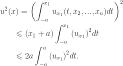 .
.
Thus
 .
.
Integration over  from
from  to
to  gives the result.
The Poincaré inequality for  spaces. Assume that
  and that is a bounded open subset of the -dimensional Euclidean space with a Lipschitz boundary (i.e., is an open, bounded Lipschitz domain). Then there exists a constant , depending only on and , such that for every function in the Sobolev space ,
 ,
,
where  is defined to be
  .
.
Proof. The proof of this version is exactly the same to the proof of case.
Remark. The point  on the boundary of is important. Otherwise, the constant function will not satisfy the Poincaré inequality. In order to avoid this restriction, a weight has been added like the classical Poincaré inequality for case. Sometimes, the Poincaré inequality for spaces is called the Sobolev inequality.


![X = [0,\frac 12 ) \cup (\frac 12, 1]](https://s0.wp.com/latex.php?latex=X+%3D+%5B0%2C%5Cfrac+12+%29+%5Ccup+%28%5Cfrac+12%2C+1%5D&bg=ffffff&fg=333333&s=0&c=20201002)


 is a normed space and
  is a set of linearly independent elements in
  such that for any
  with
with  , the all elements of
  are also linearly independent.
 with
with  with
with 

 is a reflexive Banach space and
  is a bounded sequence. Then up to a subsequence
  converges weakly to some
  in
in  between Banach spaces maps every weakly convergent sequence in
  , the Sobolev norm
  (or
(or  ) is defined by
 .
. strongly in
  , i.e.
  then
then  and
and  strongly in
  spaces. We assume
  in
in  and
and  converge weakly to
  in
in  and
and  are bounded in
  such that
 are in
  the dual space of
  -the space of test functions. It follows that
  and, hence,
  . It follows that
  and thus
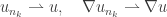
 in
in  is bounded. We shall prove that
  and
and  is bounded in
  in
in  which implies
  converges to
  (in the topological of
  contains a sub-subsequence that converges to


 . Having this and the fact that weak limit is unique we deduce that

 with Dirichlet boundary condition. We assume
  . Our aim is to show the existence of the first eigenvalue
  . Obviously, our problem is to solve the following optimization
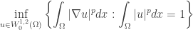 .
. contains a weakly convergent subsequence. Then
  it is clear to see that
  since
since
 .
. . It is worth noticing that by saying
  in
in  . Now we need further argument
 converges weakly, it also converges strongly. We take
  in
in  for any
  . By using the Minkowski and Holder inequalities we can show that
  , we denote its
  -dimensional Lebesgue measure by
  . We will denote by
  the open ball centered at the origin and having the same measure as
  . The norm of vector
  will be denoted by
  . Finally, we will denote by
  the
the  . It is worth recalling that
 us the usual gamma function.
 be a bounded domain. Let
  be a measurable function. Then, its Schwarz symmetrization (or the spherically symmetric and decreasing rearrangement) is the function
  defined by
 .
. is the radius of
  , then
 -dimensional Euclidean space satisfies a Hölder condition, or is Hölder continuous, when there are nonnegative real constants
  , such that
 in the domain of
  is called the exponent of the Hölder condition. If
  , then the function satisfies a Lipschitz condition. If
  , then the function simply is bounded.
 , where
  an integer, consists of those functions on
  and such that the
  . This is a locally convex topological vector space.
 ,
, be a measurable function. For
  , the level set
  is defined as
 .
. ,
,  ,
,  and so on are defined by analogy. Then the distribution function of
  .
. and for
  we have
  while for
  , we have
  . Thus the range of
  is the interval
 ![[0, |\Omega|]](https://s0.wp.com/latex.php?latex=%5B0%2C+%7C%5COmega%7C%5D&bg=ffffff&fg=333333&s=0&c=20201002) .
. , is defined on
 where
where  is non-decreasing, i.e. if
  in the sense that
  for all
  .
.![u^\sharp : [0,|\Omega|] \to \mathbb R](https://s0.wp.com/latex.php?latex=u%5E%5Csharp+%3A+%5B0%2C%7C%5COmega%7C%5D+%5Cto+%5Cmathbb+R&bg=ffffff&fg=333333&s=0&c=20201002) are equimeasurable (i.e. they have the same distribution function), i.e. for all
are equimeasurable (i.e. they have the same distribution function), i.e. for all  .
. (
( ) has a subsequence whose
  which converges weakly to an element
  such that the arithmetic means
 , is the collection of all continuous linear functionals, i.e., the set of all mapping
  satisfying
 ,
, 
 when
when  .
. in the following sense:
  is said to be open if and only if for each
  , there exists
  .
. is said to be bounded if there is a positive number
  such that
  for all
  , one has
  . Clearly,
 but
but  . This shows the lack of boundedness implies the lack of continuity.
 ;
; .
.

