This note concerns the equivalence between the three properties usually taken as an axiom in synthetic constructions of the real numbers. We start with the least upper bound property, call L, which is usually appeared in construction of the real numbers.
(L, least upper bound axiom): If  is a non-empty subset of
  , and if has an upper bound, then has a least upper bound
  , such that for every upper bound
  of , there holds
  .
.
The second property, call C, is the completeness of reals.
(C, completeness axiom): If  and
and  are non-empty subsets of with the property
  for any
  and
and  , then there is some
  such that
  for any and .
The third, also last, property, call AC, is the set of two results: the Archimedean property and Cantor’s intersection theorem. These two results often appear as consequences of the construction of reals.
Archimedean property: For any real numbers  and
and  with
with  , there exists some natural number
  such that
  .
.
Cantor’s intersection theorem: A decreasing nested sequence of non-empty, closed intervals in has a non-empty intersection.
Our aim is to prove that in fact the above three properties (L), (C), and (AC) are equivalent. Our strategy is to show the following direction:
(L) ⟶ (C) ⟶ (AC) ⟶ (L).
(more…)

![[a,b]](https://s0.wp.com/latex.php?latex=%5Ba%2Cb%5D&bg=ffffff&fg=333333&s=0&c=20201002)


![\phi \in C^1([a,b])](https://s0.wp.com/latex.php?latex=%5Cphi+%5Cin+C%5E1%28%5Ba%2Cb%5D%29&bg=ffffff&fg=333333&s=0&c=20201002)

. Then any weak solution to
 is an invertible function with inverse
  . If
. If  with
with  and
and  is continuous at
  , then
  and
and
 the set set of positive integers, namely
  .
. defined by
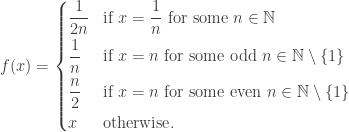
![f : [0,1] \to [0, +\infty)](https://s0.wp.com/latex.php?latex=f+%3A+%5B0%2C1%5D+%5Cto+%5B0%2C+%2B%5Cinfty%29&bg=ffffff&fg=333333&s=0&c=20201002) be a function. First, we have the following trivial result:
be a function. First, we have the following trivial result:
 , then we must have
  in
in ![[0,1]](https://s0.wp.com/latex.php?latex=%5B0%2C1%5D&bg=ffffff&fg=333333&s=0&c=20201002) .
. near zero and
 in such a way that
 ![[0,\delta]](https://s0.wp.com/latex.php?latex=%5B0%2C%5Cdelta%5D&bg=ffffff&fg=333333&s=0&c=20201002) .
. be open,
  is an arbitrary point, and
  is a function. Recall that
  if there is a linear map, denoted by
 . Notice that in the nominator of the above quotient, the symbol
  is simply the absolute value function. But this is no longer true for higher-order derivatives that we are going to define.
 is differentiable at
  exist in a neighborhood of
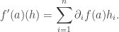
 exist in a neighborhood of
 with
with  . The two cases
  and
and  are of special because these are always mentioned in many textbooks as
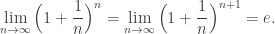
 . Hence we are left with the monotonicity of
  . When
  , as the function
  is monotone increasing with respect to
  . To study this problem, we examine
  with respect to
 ![\displaystyle f'(x) = \Big(1+\frac 1x\Big)^{x+a } \Big[ \log \Big(1+\frac 1x\Big)- \frac{x+a }{x(x+1)}\Big].](https://s0.wp.com/latex.php?latex=%5Cdisplaystyle+f%27%28x%29+%3D++%5CBig%281%2B%5Cfrac+1x%5CBig%29%5E%7Bx%2Ba+%7D+%5CBig%5B+%5Clog+%5CBig%281%2B%5Cfrac+1x%5CBig%29-+%5Cfrac%7Bx%2Ba+%7D%7Bx%28x%2B1%29%7D%5CBig%5D.&bg=ffffff&fg=333333&s=0&c=20201002)

 .
.

 is actually the normal derivative
  . Therefore, the only direction taking into derivatives of
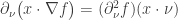


 between two metric spaces to obtain a new function
  enjoying certain properties
 and
and  respectively.
![X = [0,\frac 12 ) \cup (\frac 12, 1]](https://s0.wp.com/latex.php?latex=X+%3D+%5B0%2C%5Cfrac+12+%29+%5Ccup+%28%5Cfrac+12%2C+1%5D&bg=ffffff&fg=333333&s=0&c=20201002) and let
and let  and
and  . For example, we can choose

 of
of  . Thus, we have just shown that continuity is not enough. For this reason, we require
  be a diffeomorphism in
  . Fix a point
 denotes the open ball in
  .
. to be a
 enjoys the following properties
 be a function such that both
  are continuous in
  and
and  -plane, including
  ,
,  . Also suppose that the functions
  and
and  are both continuous and both have continuous derivatives for
 do not depend on the parameter