Mellin transform with some examples

March 31, 2009

Mellin transform with some examples

Filed under: Linh Tinh, Nghiên Cứu Khoa Học — Ngô Quốc Anh @ 13:11

In mathematics, the Mellin transform is an integral transform that may be regarded as the multiplicative version of the two-sided Laplace transform. This integral transform is closely connected to the theory of Dirichlet series, and is often used in number theory and the theory of asymptotic expansions; it is closely related to the Laplace transform and the Fourier transform, and the theory of the gamma function and allied special functions.

The Mellin transform of a function is

$\displaystyle\mathcal{M}\left\{ {f\left( x \right)} \right\}(s) = \varphi (s) = \int_0^\infty {{x^s}} f(x)\frac{{dx}} {x}$ .

The inverse transform is

$\displaystyle {\mathcal{M}^{ - 1}}\left\{ {\varphi \left( s \right)} \right\}(x) = f(x) = \frac{1} {{2\pi i}}\int_{c - i\infty }^{c + i\infty } {{x^{ - s}}} \varphi (s)ds$ .

The notation implies this is a line integral taken over a vertical line in the complex plane. Conditions under which this inversion is valid are given in the Mellin inversion theorem. The transform is named after the Finnish mathematician Hjalmar Mellin.

Importance of the fundamental strip

A Mellin transform should never be computed without its fundamental strip, which tells us where the image function converges. This strip is key to the Mellin inversion process, which arises in number theoretic applications of the transform and in the study of harmonic sums, frequently encountered in computer science. The basic idea is to compute the Mellin transform of a sum and invert it thereafter, thus obtaining an asymptotic expansion. However the Mellin inversion integral is computed over a line parallel to the imaginary axis that lies in the fundamental strip. Without knowing where the strip lies, the integral cannot be computed, more precisely, one does not know which residues contribute to its value.

The fundamental strip arises from the analysis of the convergence properties of the Mellin integral

$\displaystyle\int_0^\infty x^s f(x)\frac{dx}{x}$ .

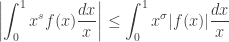
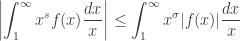
We split the integral into two parts, as follows

$\displaystyle\left( \int_0^1 + \int_1^\infty \right) x^s f(x)\frac{dx}{x}$ .

Assuming $f(x)$ is locally integrable along the positive real line, the first integral must remain bounded at zero, and the second, at infinity (understood as “in the limit” if e.g. Riemann integrability is used).

File:MellinStrip.png

Letting $s=\sigma + it$ , we find that

$\displaystyle\left| \int_0^1 x^s f(x)\frac{dx}{x} \right| \le \int_0^1 x^\sigma |f(x)| \frac{dx}{x}$

and

$\displaystyle\left| \int_1^\infty x^s f(x)\frac{dx}{x} \right| \le \int_1^\infty x^\sigma |f(x)| \frac{dx}{x}$ .

Now suppose $f(x) = O(x^u)$ at $x=0$ . The first bounding integral converges if

$\displaystyle\sigma + u - 1 > -1 \quad \mbox{or} \quad \sigma > -u$ .

Furthermore suppose that $f(x) = O(x^v)$ at infinity. The second bounding integral converges if

$\displaystyle\sigma + v - 1 < -1 \quad \mbox{or} \quad \sigma < -v$ .

These two constraints on s define two half planes, the first a left half plane and the second one a right half plane. The intersection of the two half planes is the fundamental strip, denoted $\left\langle { - u, - v} \right\rangle$ . It frequently happens that the image function can be analytically continued to the whole plane, which makes it possible to compute the inversion integral by shifting the line of integration to the left or to the right. The original Mellin integral, however, remains restricted to the fundamental strip.

Summary.

If is locally integrable along the positive real line, and

$\displaystyle f(x)_{x\rightarrow 0+} = O(x^u) \quad \mbox{and} \quad f(x)_{x\rightarrow +\infty} = O(x^v)$

then its Mellin transform converges in the fundamental strip $\left\langle { - u, - v} \right\rangle$ and the corresponding Mellin inversion integral is taken along a line parallel to the imaginary axis in this strip.

Computing the fundamental strip

As an example, consider the transform pair

$\displaystyle f(x) = \frac{1}{1+x} \quad \mbox{and} \quad \varphi(s) = \frac{\pi}{\sin \pi s}$ .

By inspection, we have

$\displaystyle f(x)_{x\rightarrow 0+} = O(1) = O(x^0)$

and

$\displaystyle f(x)_{x\rightarrow +\infty} \sim \frac{1}{x} = O(x^{-1})$

and the fundamental strip is $\left\langle { 0, 1} \right\rangle$ . This is illustrated in the first diagram at the beginning of this section.

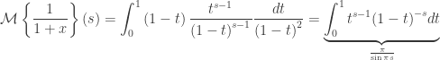
As a second example, consider the transform pair

$\displaystyle f(x) = \exp(-x) -1 + x \quad \mbox{and} \quad \varphi(s) = \Gamma(s)$ .

We have the following series expansion around

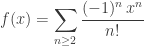
$\displaystyle f(x) = \sum_{n\ge 2} \frac{(-1)^n \, x^n}{n!}$ ,

which implies that

$\displaystyle f(x)_{x\rightarrow 0+} = O(x^2)$ .

At infinity, we have

$\displaystyle f(x)_{x\rightarrow +\infty} \sim x = O(x^1)$

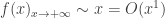
so that the fundamental strip is $\left\langle { - 2, - 1} \right\rangle$ . This is shown in the second diagram.

Some relation

Gamma function: Clearly,

$\displaystyle\mathcal M\left\{ {{e^{ - ax}}u\left( x \right)} \right\}\left( s \right) = \int_0^\infty {{e^{ - ax}}{x^{s - 1}}dx} = {a^{ - s}}\Gamma \left( s \right)$ .

Relation to Laplace Transform: By letting , the transform becomes

$\displaystyle\mathcal M\left\{ {f\left( x \right)} \right\}\left( s \right) = \int_{ - \infty }^\infty {f\left( {{e^{ - t}}} \right){e^{ - st}}dt} = \mathcal L\left\{ {f\left( {{e^{ - t}}} \right)} \right\}\left( s \right)$ .

Relation to Fourier Transform: By setting we obtain

$\displaystyle M\left\{ {f\left( x \right)} \right\}\left( {s = \sigma + j2\pi \beta } \right) = L\left\{ {f\left( {{e^{ - t}}} \right){e^{ - \sigma t}}} \right\}\left( \beta \right)$ .

Properties of Mellin Transform

Scaling Property

$\displaystyle\mathcal{M}\left\{ {f\left( {ax} \right)} \right\}\left( s \right) = \int_{ - \infty }^\infty {f\left( {ax} \right){x^{s - 1}}dx} = {a^{ - s}}\underbrace {\int_{ - \infty }^\infty {f\left( x \right){x^{s - 1}}dx} }_{\mathcal{M}\left\{ {f\left( x \right)} \right\}\left( s \right)}$ .

Multiplication by

$\displaystyle\mathcal{M}\left\{ {{x^a}f\left( x \right)} \right\}\left( s \right) = \int_{ - \infty }^\infty {f\left( x \right){x^{\left( {a + s} \right) - 1}}dx} = \mathcal{M}\left\{ {f\left( x \right)} \right\}\left( {s + a} \right)$ .

Raising the Independent Variable to a Real Power

$\displaystyle\mathcal{M}\left\{ {f\left( {{x^a}} \right)} \right\}\left( s \right) = \int_{ - \infty }^\infty {f\left( {{x^a}} \right){x^{s - 1}}dx} = \underbrace {\int_{ - \infty }^\infty {f\left( x \right){x^{\frac{s} {a} - \frac{1} {a}}}\left( {\frac{1} {a}{x^{\frac{1} {a} - 1}}dx} \right)} }_{\mathcal{M}\left\{ {f\left( x \right)} \right\}\left( {\frac{s} {a}} \right),\quad a > 0}$

Inverse of Independent Variable

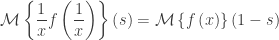
$\displaystyle\mathcal{M}\left\{ {\frac{1} {x}f\left( {\frac{1} {x}} \right)} \right\}\left( s \right) = \mathcal{M}\left\{ {f\left( x \right)} \right\}\left( {1 - s} \right)$ .

Multiplication by

$\displaystyle\mathcal{M}\left\{ {\left( {\ln x} \right)f\left( x \right)} \right\}\left( s \right) = \frac{d} {{ds}}\mathcal{M}\left\{ {f\left( x \right)} \right\}\left( s \right)$ .

Multiplication by a Power of

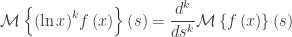
$\displaystyle\mathcal{M}\left\{ {{{\left( {\ln x} \right)}^k}f\left( x \right)} \right\}\left( s \right) = \frac{{{d^k}}} {{d{s^k}}}\mathcal{M}\left\{ {f\left( x \right)} \right\}\left( s \right)$ .

Derivative

$\displaystyle\mathcal{M}\left\{ {\frac{{{d^k}}} {{d{x^k}}}f\left( x \right)} \right\}\left( s \right) = {\left( { - 1} \right)^k}\frac{{\Gamma \left( s \right)}} {{\Gamma \left( {s - k} \right)}}\mathcal{M}\left\{ {f\left( x \right)} \right\}\left( {s - k} \right)$ .

Derivative Multiplied by Independent Variable

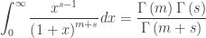
$\displaystyle\mathcal{M}\left\{ {{x^k}\frac{{{d^k}}} {{d{x^k}}}f\left( x \right)} \right\}\left( s \right) = {\left( { - 1} \right)^k}\frac{{\Gamma \left( {s + k} \right)}} {{\Gamma \left( s \right)}}\mathcal{M}\left\{ {f\left( x \right)} \right\}\left( s \right)$ .

Convolution

$\displaystyle\mathcal{M}\left\{ {f\left( x \right)g\left( x \right)} \right\}\left( s \right) = \frac{1} {{2\pi i}}\int_{c - i\infty }^{c + i\infty } {\mathcal{M}\left\{ {f\left( x \right)} \right\}\left( z \right)\mathcal{M}\left\{ {g\left( x \right)} \right\}\left( {s - z} \right)dz}$ .

Multiplicative Convolution

$\displaystyle\begin{gathered} \mathcal{M}\left\{ {f\left( x \right) \vee g\left( x \right)} \right\}\left( s \right) = \mathcal{M}\left\{ {f\left( x \right)} \right\}\left( s \right)\mathcal{M}\left\{ {g\left( x \right)} \right\}\left( s \right), \hfill \\ {\mathcal{M}^{ - 1}}\left( {\mathcal{M}\left\{ {f\left( x \right)} \right\}\left( s \right)\mathcal{M}\left\{ {g\left( x \right)} \right\}\left( s \right)} \right)\left( x \right) = \int_0^\infty {f\left( {\frac{x} {u}} \right)g\left( u \right)\frac{{du}} {u}.} \hfill \\ \end{gathered}$

Examples of Mellin Transform

Characteristic function.

$\displaystyle\mathcal{M}\left\{ {{x^a}{\chi _{\left[ {{x_0},\infty } \right)}}\left( x \right)} \right\}\left( s \right) = \int_{{x_0}}^\infty {{x^{{x_0} + s - 1}}dx} = - \frac{{x_0^{a + s}}} {{a + s}},\quad \Re e x < - a$ .

Fractional function.

$\displaystyle\mathcal{M}\left\{ {\frac{1} {{1 + x}}} \right\}\left( s \right) = \int_0^\infty {\frac{{{x^{s - 1}}}} {{1 + x}}dx}$ .

Setting we obtain and

$\displaystyle dt = \frac{{dx}} {{{{\left( {1 + x} \right)}^2}}}$ .

Therefore,

$\displaystyle\mathcal{M}\left\{ {\frac{1} {{1 + x}}} \right\}\left( s \right) = \int_0^1 {\left( {1 - t} \right)\frac{{{t^{s - 1}}}} {{{{\left( {1 - t} \right)}^{s - 1}}}}\frac{{dt}} {{{{\left( {1 - t} \right)}^2}}}} = \underbrace {\int_0^1 {{t^{s - 1}}{{\left( {1 - t} \right)}^{ - s}}dt} }_{\frac{\pi } {{\sin \pi s}}}$ .

Polynomial function.

From

$\displaystyle\int_0^1 {{{\left( {1 - u} \right)}^{m - 1}}{u^{s - 1}}du} = \frac{{\Gamma \left( m \right)\Gamma \left( s \right)}} {{\Gamma \left( {m + s} \right)}}, \quad \Re e s > 0, \Re e m > 0$

with the setting , we obtain

$\displaystyle\int_0^\infty {\frac{{{x^{s - 1}}}} {{{{\left( {1 + x} \right)}^{m + s}}}}dx} = \frac{{\Gamma \left( m \right)\Gamma \left( s \right)}} {{\Gamma \left( {m + s} \right)}}$ .

Hence

$\displaystyle\mathcal{M}\left\{ {{{\left( {\frac{1} {{1 + x}}} \right)}^a}} \right\}\left( s \right) = \frac{{\Gamma \left( s \right)\Gamma \left( {a - s} \right)}} {{\Gamma \left( a \right)}}, \quad 0 < \Re e s < \Re e a$ .

Source

Comments (12)

12 Comments »

great write up; could you point me to a reference with proofs?
also, it is not clear how to define f wedge g?

Comment by here — December 2, 2010 @ 10:58

Reply
- Hi, thanks for your interest in my blog. For your question, feel free to check the following document
  
  Click to access MELLIN.pdf
  
  Happy reading.
  
  Comment by Ngô Quốc Anh — December 2, 2010 @ 12:07
  
  Reply
hi thanks for the write up. I am very new to this transform. It is being very hard for me to understand the math. Can u guide me to a resource where it is explained in more detailed and a simple manner.

thanks.

Comment by Raja sekhar — August 16, 2012 @ 2:12

Reply
Hi. Good article. One property you did not mention is that Mellin transform of the product of independent random variables equals the product of their Mellin transforms.
Also, can you guide me is there any way to determine the Characteristic function of a random variable from its Mellin transform? Thanks.

Comment by Sohail — November 18, 2012 @ 21:22

Reply
plz can sumone give proof of mellin of error function…….

Comment by sara — November 12, 2013 @ 23:37

Reply
- Thanks. What kind of error functions are you talking about?
  
  Comment by Ngô Quốc Anh — November 12, 2013 @ 23:38
  
  Reply
  - erf(at)=[ 2/sqrt(pi)]
    *limit of integration(0 to at) exp(-u^2) du
    
    Comment by sara — November 13, 2013 @ 0:09
  - It should be well-known, check the third one from the bottom 😉 http://mathworld.wolfram.com/MellinTransform.html
    
    Comment by Ngô Quốc Anh — November 13, 2013 @ 0:10
  - thanks sir. but i actualy want its proof?
    
    Comment by sara — November 13, 2013 @ 0:13
  - the solution steps for this rzlt ???
    
    Comment by sara — November 13, 2013 @ 0:14
  - I don’t think it is difficult, just a time consuming 😉 Show me your working, maybe I can help you at some point.
    
    Comment by Ngô Quốc Anh — November 13, 2013 @ 0:26
erf(at)=[ 2/sqrt(pi)]
*limit of integration(0 to at) exp(-u^2) du

Comment by sara — November 13, 2013 @ 0:02

Reply

RSS feed for comments on this post. TrackBack URI

	Earth Salt and Space… on Stereographic projection
	Ngô Quốc Anh on Extending functions between me…
	Why does Paneitz ope… on Conformal Changes of Riemannia…
	Ngô Quốc Anh on Conformal Changes of Riemannia…
	NT Tài on Conformal Changes of Riemannia…
	Calculating scalar c… on Conformal change of the Laplac…
	Poincare inequality?… on The Poincaré inequality: W^{1,…
	Implicit function th… on The implicit function theorem:…
	Heuristics for the Y… on The Yamabe problem: A Sto…
	Is there a reference… on Compact embedding of Hölder…

Ngô Quốc Anh

March 31, 2009