What is a gradient flow?

November 5, 2010

What is a gradient flow?

Filed under: Uncategorized — Tags: flow — Ngô Quốc Anh @ 18:40

In this entry, we shall discuss the following question: “What is a gradient flow?”.

Let $(H, \langle {\cdot, \cdot}\rangle)$ be a Hilbert space with norm $\| \cdot\|$ . Let $\phi$ be a convex, lower semi-continuous functional defined on a dense domain $\text{Dom}(\phi) \subset H$ .

Definition. The subdifferential of $\phi$ at a point $u \in \text{Dom}(\phi)$ is the set $\partial \phi(u) \subset H$ defined by

$\partial \phi (u) =\{p \in H: \phi(v) \geqslant \phi(u)+\langle p, v-u\rangle \quad \forall v \in \text{Dom}(\phi)\}$ .

Vector $p$ is called subgradient at $u$ , thus, the set of all subgradients at $u$ is called the subdifferential at $u$ .

The geometric meaning of subdifferential is as the set of all possible “slopes” of affine hyperplanes touching the graph of $\phi$ from below at the point $u$ . Thus, $\phi$ is differentiable at $u$ iff its subdifferential at $u$ contains exactly one vector as its derivative at that point.

We now recall the classical definition of gradient flow on a Hilbert space.

Definition. A function $u\in AC_{loc}((0,+\infty); H)$ , the class of absolutely continuous from $(0,+\infty)$ to $H$ , is a gradient flow of the convex, lower semi-continuous functional $\phi$ iff the differential inclusion

$u_t \in -\partial \phi(u(t))$

is satisfied almost everywhere with respect to $t$ .

In practice for a given flow

$u_t = F(u)$ ,

if $\phi$ is differentiable and is given as an integral over some domain, say, $\Omega$ , we simply verify there is some number $\lambda$ so that

$\displaystyle \int_\Omega u_t F(u) = \lambda \frac{d}{dt}\phi(u(t))$ .

If $\lambda >0$ , the flow is called positive gradient flow. Now we discuss some examples.

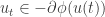
Example 1. The following semilinear heat equation

$u_t =\Delta u+|u|^{2^\star-1}, \quad x \in \Omega$

corresponds formally to the $L^2$ gradient flow associated to the energy functional

$\displaystyle E(u)=\frac{1}{2}\int_\Omega |\nabla u|^2dx-\frac{1}{2^\star}\int_\Omega |u|^{2^\star}dx$ .

Here we assume the boundary and initial conditions are all zero just for simplicity.

Observe that

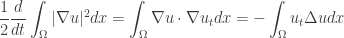
$\displaystyle\frac{1}{2}\frac{d}{{dt}}\int_\Omega {|\nabla u{|^2}dx} = \int_\Omega {\nabla u \cdot \nabla {u_t}dx} = - \int_\Omega {{u_t}\Delta udx}$

and

$\displaystyle\frac{1}{{{2^ \star }}}\frac{d}{{dt}}\int_\Omega | u{|^{{2^ \star }}}dx = \int_\Omega | u{|^{{2^ \star } - 1}}{u_t}dx$ .

Therefore

$\displaystyle\frac{d}{{dt}}E(u) = - \int_\Omega {{u_t}\left[ {\Delta u + |u{|^{{2^ \star } - 1}}} \right]dx}$

i.e.

$\displaystyle u_t =\Delta u+u^{2^\star-1}$

is the $L^2$ gradient flow associated to the energy functional

$\displaystyle E(u)=\frac{1}{2}\int_\Omega |\nabla u|^2dx-\frac{1}{2^\star}\int_\Omega |u|^{2^\star}dx$ .

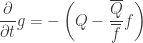
Example 2. Heat flow for Nirenberg’s problem

$u_t = \alpha f - K$

is also a gradient flow for the following functional

$\displaystyle E_f(u)=\int_{\mathbb S^2} (|\nabla u|^2+2u)dv_g - \log\left(\int_{\mathbb S^2} fe^{2u}dv_g\right)$ .

For the details of this flow, we refer the reader to a paper due to Michael Struwe published in Duke Math. J. in 2005 [here].

Example 3. $Q$ -curvature flow

$\displaystyle \frac{\partial}{\partial t}g=-\left(Q-\frac{\overline Q}{\overline f}f\right)$

is a gradient flow for some functional. For details, we refer the reader to a paper due to Simon Brendle published in Ann. of Math. in 2003 [here].

Source: Steepest descent flows and applications to spaces of probability measures by Luigi Ambrosio.

Comments (1)

1 Comment »

[…] E[u]=int w(u)+epsilon ^2 |nabla u|^2 ) $$ I tried to follow the definition of gradient flow from : https://anhngq.wordpress.com/2010/11/05/what-is-a-gradient-flow/ but I got stucked and […]

Pingback by gradient flow -cahn hilliard - MathHub — May 14, 2016 @ 17:50

Reply

RSS feed for comments on this post. TrackBack URI

M	T	W	T	F	S	S
1	2	3	4	5	6	7
8	9	10	11	12	13	14
15	16	17	18	19	20	21
22	23	24	25	26	27	28
29	30

	Earth Salt and Space… on Stereographic projection
	Ngô Quốc Anh on Extending functions between me…
	Why does Paneitz ope… on Conformal Changes of Riemannia…
	Ngô Quốc Anh on Conformal Changes of Riemannia…
	NT Tài on Conformal Changes of Riemannia…
	Calculating scalar c… on Conformal change of the Laplac…
	Poincare inequality?… on The Poincaré inequality: W^{1,…
	Implicit function th… on The implicit function theorem:…
	Heuristics for the Y… on The Yamabe problem: A Sto…
	Is there a reference… on Compact embedding of Hölder…

Ngô Quốc Anh

November 5, 2010